WIXLIB

Introduction to Machine LearningFiguresEthem Alpaydınc The MIT Press, 2004 1

Chapter 1:Introduction2

Savingsθ2Low-RiskHigh-RiskIncomeθ1Figure 1.1: Example of a training dataset where eachcircle corresponds to one data instance with inputvalues in the corresponding axes and its signindicates the class. For simplicity, only two customerattributes, income and savings, are taken as inputand the two classes are low-risk (‘ ’) and high-risk(‘ ’). An example discriminant that separates thetwo types of examples is also shown. From:E. Alpaydın. 2004. Introduction to MachinecLearning. TheMIT Press.3

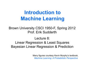
y: pricex: milageFigure 1.2: A training dataset of used cars and thefunction fitted. For simplicity, milage is taken as theonly input attribute and a linear model is used.From: E. Alpaydın. 2004. Introduction to MachinecLearning. TheMIT Press.4

Chapter 2:Supervised Learning5

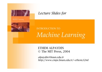
x2: Engine powerx2tx1tx1: PriceFigure 2.1: Training set for the class of a “familycar.” Each data point corresponds to one examplecar and the coordinates of the point indicate theprice and engine power of that car. ‘ ’ denotes apositive example of the class (a family car), and ‘ ’denotes a negative example (not a family car); it isanother type of car. From: E. Alpaydın. 2004.cIntroduction to Machine Learning. TheMIT Press.6

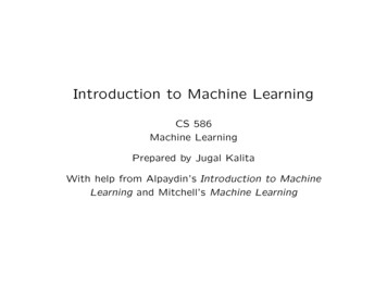
x2: Engine powerCe2e1p1p2x1: PriceFigure 2.2: Example of a hypothesis class. The classof family car is a rectangle in the price-engine powerspace. From: E. Alpaydın. 2004. Introduction tocMachine Learning. TheMIT Press.7

x2: Engine powere2e1?False positivehCp1p2False negativex1: PriceFigure 2.3: C is the actual class and h is our inducedhypothesis. The point where C is 1 but h is 0 is afalse negative, and the point where C is 0 but h is 1is a false positive. Other points, namely truepositives and true negatives, are correctly classified.From: E. Alpaydın. 2004. Introduction to MachinecLearning. TheMIT Press.8

x2: Engine powerGCSx1: PriceFigure 2.4: S is the most specific hypothesis and G isthe most general hypothesis. From: E. Alpaydın.c2004. Introduction to Machine Learning. TheMITPress.9

x2x1Figure 2.5: An axis-aligned rectangle can shatterfour points. Only rectangles covering two points areshown. From: E. Alpaydın. 2004. Introduction tocMachine Learning. TheMIT Press.10

x2Chx1Figure 2.6: The difference between h and C is thesum of four rectangular strips, one of which isshaded. From: E. Alpaydın. 2004. Introduction tocMachine Learning. TheMIT Press.11

x2h2h1x1Figure 2.7: When there is noise, there is not a simpleboundary between the positive and negativeinstances, and zero misclassification error may not bepossible with a simple hypothesis. A rectangle is asimple hypothesis with four parameters defining thecorners. An arbitrary closed form can be drawn bypiecewise functions with a larger number of controlpoints. From: E. Alpaydın. 2004. Introduction tocMachine Learning. TheMIT Press.12

Engine powerSports car?Luxury sedanFamily carPriceFigure 2.8: There are three classes: family car, sportscar, and luxury sedan. There are three hypothesesinduced, each one covering the instances of one classand leaving outside the instances of the other twoclasses. ‘?’ are reject regions where no, or more thanone, class is chosen. From: E. Alpaydın. 2004.cIntroduction to Machine Learning. TheMIT Press.13

y: pricex: milageFigure 2.9: Linear, second-order, and sixth-orderpolynomials are fitted to the same set of points. Thehighest order gives a perfect fit but given this muchdata, it is very unlikely that the real curve is soshaped. The second order seems better than thelinear fit in capturing the trend in the training data.From: E. Alpaydın. 2004. Introduction to MachinecLearning. TheMIT Press.14

Chapter 3:Bayes Decision Theory15

x2C1rejectC2C3x1Figure 3.1: Example of decision regions and decisionboundaries. From: E. Alpaydın. 2004. Introductioncto Machine Learning. TheMIT Press.16

RainP(R) 0.4Wet grassP(W R) 0.9P(W R) 0.2Figure 3.2: Bayesian network modeling that rain isthe cause of wet grass. From: E. Alpaydın. 2004.cIntroduction to Machine Learning. TheMIT Press.17

P(S) 0.2P(R) 0.4SprinklerRainWet grassP(W R,S) 0.95P(W R, S) 0.90P(W R,S) 0.90P(W R, S) 0.10Figure 3.3: Rain and sprinkler are the two causes ofwet grass. From: E. Alpaydın. 2004. Introduction tocMachine Learning. TheMIT Press.18

P(C) 0.5CloudyP(S C) 0.1P(S C) 0.5P(R C) 0.8P(R C) 0.1SprinklerRainWet grassP(W R,S) 0.95P(W R, S) 0.90P(W R,S) 0.90P(W R, S) 0.10Figure 3.4: If it is cloudy, it is likely that it will rainand we will not use the sprinkler. From: E. Alpaydın.c2004. Introduction to Machine Learning. TheMITPress.19

P(C) 0.5CloudyP(S C) 0.1P(S C) 0.5P(R C) 0.8P(R C) 0.1SprinklerRainP(W R,S) 0.95P(W R, S) 0.90P(W R,S) 0.90P(W R, S) 0.10P(F R) 0.1P(F R) 0.7Wet grassrooFFigure 3.5: Rain not only makes the grass wet butalso disturbs the cat who normally makes noise onthe roof. From: E. Alpaydın. 2004. Introduction tocMachine Learning. TheMIT Press.20

P(C)Cp(x C)xFigure 3.6: Bayesian network for classification.From: E. Alpaydın. 2004. Introduction to MachinecLearning. TheMIT Press.21

P(C)Cp(x1 C)p(xd C)p(x2 C)x1x2xdFigure 3.7: Naive Bayes’ classifier is a Bayesiannetwork for classification assuming independentinputs. From: E. Alpaydın. 2004. Introduction tocMachine Learning. TheMIT Press.22

chooseclassxUFigure 3.8: Influence diagram corresponding toclassification. Depending on input x, a class ischosen that incurs a certain utility (risk). From:E. Alpaydın. 2004. Introduction to MachinecLearning. TheMIT Press.23

Chapter 4:Parametric Methods24

variancediE[d]θbiasFigure 4.1: θ is the parameter to be estimated. diare several estimates (denoted by ‘ ’) over differentsamples. Bias is the difference between the expectedvalue of d and θ. Variance is how much di arescattered around the expected value. We would likeboth to be small. From: E. Alpaydın. 2004.cIntroduction to Machine Learning. TheMIT Press.25

Likelihoods0.4p(x Ci)0.30.20.10 10 8 6 4 20x24681046810Posteriors with equal priors10.8p(Ci x)0.60.40.20 10 8 6 4 20x2Figure 4.2: Likelihood functions and the posteriorswith equal priors for two classes when the input isone-dimensional. Variances are equal and theposteriors intersect at one point, which is thethreshold of decision. From: E. Alpaydın. 2004.cIntroduction to Machine Learning. TheMIT Press.26

Likelihoods0.4p(x Ci)0.30.20.10 10 8 6 4 20x24681046810Posteriors with equal priors10.8p(Ci x)0.60.40.20 10 8 6 4 20x2Figure 4.3: Likelihood functions and the posteriorswith equal priors for two classes when the input isone-dimensional. Variances are unequal and theposteriors intersect at two points. From:E. Alpaydın. 2004. Introduction to MachinecLearning. TheMIT Press.27

E[R x] wx w 0E[R x*]p(r x*)x*XFigure 4.4: Regression assumes 0 mean Gaussiannoise added to the model; here, the model is linear.From: E. Alpaydın. 2004. Introduction to MachinecLearning. TheMIT Press.28

(a) Function and data(b) Order 15500 501234 5501(c) Order 3500012334545(d) Order 55 524 550123Figure 4.5: (a) Function, f (x) 2 sin(1.5x), and onenoisy (N (0, 1)) dataset sampled from the function.Five samples are taken, each containing twentyinstances. (b), (c), (d) are five polynomial fits, gi (·),of order 1, 3, and 5. For each case, dotted line is theaverage of the five fits, namely, g(·). From:E. Alpaydın. 2004. Introduction to MachinecLearning. TheMIT Press.29

5Figure 4.6: In the same setting as that of figure 4.5,using one hundred models instead of five, bias,variance, and error for polynomials of order 1 to 5.Order 1 has the smallest variance. Order 5 has thesmallest bias. As the order is increased, biasdecreases but variance increases. Order 3 has theminimum error. From: E. Alpaydın. 2004.cIntroduction to Machine Learning. TheMIT Press.30

(a) Data and fitted polynomials50 500.511.522.533.544.55(b) Error vs polynomial order3TrainingValidation2.521.510.512345678Figure 4.7: In the same setting as that of figure 4.5,training and validation sets (each containing 50instances) are generated. (a) Training data andfitted polynomials of order from 1 to 8. (b) Trainingand validation errors as a function of the polynomialorder. The “elbow” is at 3.From: E. Alpaydın.c2004. Introduction to Machine Learning. TheMITPress.31

Chapter 5:Multivariate Methods32

0.40.350.30.250.20.150.10.050x2x1Figure 5.1: Bivariate normal distribution. From:E. Alpaydın. 2004. Introduction to MachinecLearning. TheMIT Press.33

Cov(x1,x2) 0, Var(x1) Var(x2)x2Cov(x1,x2) 0, Var(x1) Var(x2)x1Cov(x1,x2) 0Cov(x1,x2) 0Figure 5.2: Isoprobability contour plot of thebivariate normal distribution. Its center is given bythe mean, and its shape and orientation depend onthe covariance matrix. From: E. Alpaydın. 2004.cIntroduction to Machine Learning. TheMIT Press.34

p( x C1)0.10.050x2x1x2x1p(C1 x)10.50Figure 5.3: Classes have different covariancematrices. From: E. Alpaydın. 2004. Introduction tocMachine Learning. TheMIT Press.35

Figure 5.4: Covariances may be arbitary but sharedby both classes. From: E. Alpaydın. 2004.cIntroduction to Machine Learning. TheMIT Press.36

Figure 5.5: All classes have equal, diagonalcovariance matrices but variances are not equal.From: E. Alpaydın. 2004. Introduction to MachinecLearning. TheMIT Press.37

Figure 5.6: All classes have equal, diagonalcovariance matrices of equal variances on bothdimensions. From: E. Alpaydın. 2004. Introductioncto Machine Learning. TheMIT Press.38

Chapter 6:Dimensionality Reduction39

z2x2z1z2x1z1Figure 6.1: Principal components analysis centersthe sample and then rotates the axes to line up withthe directions of highest variance. If the variance onz2 is too small, it can be ignored and we havedimensionality reduction from two to one. From:E. Alpaydın. 2004. Introduction to MachinecLearning. TheMIT Press.40

(a) Scree graph for 6070506070(b) Proportion of variance explained1Prop of var0.80.60.40.20010203040EigenvectorsFigure 6.2: (a) Scree graph. (b) Proportion ofvariance explained is given for the Optdigits datasetfrom the UCI Repository. This is a handwritten digitdataset with ten classes and sixty-four dimensionalinputs. The first twenty eigenvectors explain 90percent of the variance. From: E. Alpaydın. 2004.cIntroduction to Machine Learning. TheMIT Press.41

Optdigits after PCA302203333Second Eigenvector331003777777 10 2037798792292 222322 5 32388 5 58885 8 57 99971 1119141197494 1 91449 4482180000 1 20 10606 666666444 30 30004 40 40000First Eigenvector104203040Figure 6.3: Optdigits data plotted in the space oftwo principal components. Only the labels ofhundred data points are shown to minimize theink-to-noise ratio. From: E. Alpaydın. 2004.cIntroduction to Machine Learning. TheMIT Press.42

esz1z2x1zkPCAx2xdFAFigure 6.4: Principal components analysis generatesnew variables that are linear combinations of theoriginal input variables. In factor analysis, however,we posit that there are factors that when linearlycombined generate the input variables. From:E. Alpaydın. 2004. Introduction to MachinecLearning. TheMIT Press.43

x2z2z1x1Figure 6.5: Factors are independent unit normalsthat are stretched, rotated, and translated to makeup the inputs. From: E. Alpaydın. 2004.cIntroduction to Machine Learning. TheMIT Press.44

is0Zurich 500LisbonMadrid 1000IstanbulRome 1500 2000 2500Athens 2000 1500 1000 5000500100015002000Figure 6.6: Map of Europe drawn by MDS. Citiesinclude Athens, Berlin, Dublin, Helsinki, Istanbul,Lisbon, London, Madrid, Moscow, Paris, Rome, andZurich. Pairwise road travel distances between thesecities are given as input, and MDS places them in twodimensions such that these distances are preserved aswell as possible. From: E. Alpaydın. 2004.cIntroduction to Machine Learning. TheMIT Press.45

x2m2m1m2s2 2wm1s1 2x1Figure 6.7: Two-dimensional, two-class dataprojected on w. From: E. Alpaydın. 2004.cIntroduction to Machine Learning. TheMIT Press.46