WIXLIB

Baechi: Fast Device Placement of Machine Learning Graphs2NEW ALGORITHMS FORMEMORY-CONSTRAINED PLACEMENTWe present the problem formulation and our three placementtechniques. For each technique, we first discuss the classical approach (not memory-aware), and then our adaptedmemory-constrained algorithm. Where applicable, we proveoptimality.Our three approaches are: 1) a placer based on topologicalsorting (TOPO) 2) a placer based on Earliest Task First (ETF),and 3) a placer based on Small Communication Time (SCT).2.1Problem FormulationGiven 𝑚 devices (GPUs), each with memory size 𝑀, and aMachine Learning (ML) graph 𝐺 that is a DAG (DirectedAcyclic Graph) of operators, the device placement problemis to place nodes of 𝐺 (operators) on the devices so that themakespan is minimized. Makespan, equivalent to step time,is traditionally defined as the total execution time to trainon one input mini-batch (i.e., unit of training data). Table 1summarizes key terms used throughout the paper. Whendiscussing classical algorithms, we use the classical terms“tasks” instead of operators.If one assumes devices have infinite (sufficient) memory,scheduling with communication delay is a well-studied theoretical problem. The problem is NP-hard even when underthe simplest of assumptions [19], such as infinite number ofdevices and unit times for computation and communication.Out of the three best-performing solutions to the infinitememory problem, we choose the two that map best to MLgraphs: 1) Earliest Task First or ETF [21, 49], and 2) SmallCommunication Time or SCT [17]. SCT is provably close tooptimal when the ratio of maximum communication timebetween any two tasks to minimum computation time forany task is 1. We excluded a third solution, UET-UCT [37],since it assumes unit computation and communication times,but ML graphs have heterogeneous operators.2.2m-TOPO: Topological Sort PlacerBackground: Topological Sort (Not Memory-Aware). Topological sort [25] is a linear ordering of vertices in a DAG, suchthat for each directed edge 𝑢 𝑣, 𝑢 appears before 𝑣 in thelinear ordering.New Memory-Constrained Version (m-TOPO). Our modified version, called m-TOPO, works as follows. It calculatesthe maximum load-balanced memory that will be used perdevice, by dividing total required memory by number of devices, and then accounting for outlierÍ operators. Concretely,this per-device cap is 𝐶𝑎𝑝 ( 𝑖 [𝑛] 𝑑𝑖 /𝑚 max𝑖 [𝑛] 𝑑𝑖 ).Then m-TOPO works iteratively, and assigns operators todevices in increasing order of device ID. For the currentSoCC ’20, October 19–21, 2020, Virtual Event, USAdevice, m-TOPO places operators until the device memoryusage reaches 𝐶𝑎𝑝. At that point, m-TOPO moves on to thenext device ID, and so on. At runtime, m-TOPO executes theoperators at a device in the topologically sorted order.2.3m-ETF: Earliest Task First PlacerBackground: ETF (Not Memory-Aware). ETF [21] maintains two lists: a sorted task list 𝐼 containing unscheduledtasks, and a device list 𝑃. In 𝐼 , tasks are sorted by earliestschedulable time. The earliest schedulable time of task 𝑖 isthe latest finish time of 𝑖’s parents in the DAG, plus timefor their data to reach 𝑖. In 𝑃, each device is associated withits earliest available time, i.e., last finish time of its assignedtasks (so far).ETF iteratively: i) places the head of the task queue 𝐼 at thatdevice from 𝑃 which has the earliest available time, ii) thenupdates the earliest available time of that device to be thecompletion time of the placed task, and iii) updates earliestschedulable time of that task’s dependencies in queue 𝐼 (ifapplicable).The earliest schedulable time of task 𝑗 on device 𝑝 isthe later of two times: (i) device 𝑝’s earliest available time(𝑓 𝑟𝑒𝑒 (𝑝)), and (ii) all predecessor tasks of 𝑗 have completedand have communicated their data to 𝑗. More formally, let:a) Γ ( 𝑗) be the set of 𝑗’s predecessors; b) for 𝑖: start time is𝑠𝑖 , computation time is 𝑘𝑖 ; c) 𝑥𝑖𝑝 0 when task 𝑖 is on device𝑝, otherwise 𝑥𝑖𝑝 1. Then, the earliest schedulable time oftask 𝑗 across all devices is:h imin max 𝑓 𝑟𝑒𝑒 (𝑝), max(𝑠 𝑘 𝑐𝑥).(1)𝑖𝑖𝑖𝑗𝑖𝑝 𝑝 𝑃𝑖 Γ ( 𝑗)Under the SCT assumption (Table 1), ETF’s makespanwas shown [21] to have an approximation ratio of (2 𝜌 1𝑚 ) within optimal, where 𝜌 is the ratio of the maximumcommunication time to minimum computation time, and 𝑚 isthe number of devices. This approximation ratio approaches3 when 𝜌 approaches 1 and 𝑚 1.New Memory-Constrained Version (m-ETF). Our newmodified algorithm, called m-ETF, maintains a queue 𝑄 ofoperator-device pairs (𝑖, 𝑝) for all unscheduled operatorsand all devices. Elements (𝑖, 𝑝) in 𝑄 are sorted in increasing order of the earliest schedulable time for operator 𝑖 ondevice 𝑝. This earliest schedulable time takes into accountdependent parents of 𝑖 as well as the earliest time that device𝑝 is available, given operators already scheduled at 𝑝. Thereader will notice that m-ETF’s modified queue can also beused for ETF–the key reason to use (𝑖, 𝑝) pairs is for m-ETFto do fast searches, since the earliest available device(s) mayhave insufficient memory.m-ETF iteratively looks at the head of the queue. If thehead element (𝑖, 𝑝) is not schedulable because device 𝑝’s

SoCC ’20, October 19–21, 2020, Virtual Event, USAJeon et al.leftover memory is insufficient, then the head is removed. Ifthe head is schedulable, then operator 𝑖 is assigned to starton device 𝑝 at that earliest time, and we: i) update 𝑝’s earliestavailable time to be the completion time of 𝑖, and ii) update𝑖’s child operators’ earliest schedulable times in queue 𝑄 (ifapplicable).2.4m-SCT: Small Communication TimePlacerBackground: SCT (Not Memory-Aware). The classical SCTalgorithm [17] first develops a solution assuming an infinitenumber of available devices, and then specializes for a finitenumber of devices. We elaborate details, as they are relevantto our memory-constrained version.Classical SCT: Infinite Number of Devices. SCT uses integer linear programming (ILP). The key idea is to find thefavorite child of a given task 𝑖, and prioritize its schedulingon the same device as task 𝑖. For a task 𝑖, denote its favoritechild as 𝑓 (𝑖).The original ILP specification from [17] solves for variables𝑥𝑖 𝑗 {0, 1}, where 𝑥𝑖 𝑗 0 if and only if 𝑗 is 𝑖’s favoritechild. For completeness, we provide this full ILP specificationbelow [17] (Section 3.2 in that paper). Below, the machinelearning graph is 𝐺 (𝑉 , 𝐸); and 𝑖, 𝑗 refer to operators. min 𝑤 𝑖 𝑗 𝐸 (𝐺), 𝑥𝑖 𝑗 {0, 1} 𝑖 𝑉 (𝐺), 𝑠𝑖 0 𝑖 𝑉 (𝐺), 𝑠𝑖 𝑘𝑖 𝑤 𝑖 𝑗 𝐸 (𝐺), 𝑠𝑖 𝑘𝑖 𝑐𝑖 𝑗 𝑥𝑖 𝑗 𝑠 𝑗 Õ 𝑖 𝑉 (𝐺),𝑥𝑖 𝑗 Γ (𝑖) 1 (𝑖 )𝑗 Γ Õ 𝑖 𝑉 (𝐺),𝑥𝑖 𝑗 Γ (𝑖) 1 𝑗 Γ (𝑖 ) Minimize makespan.𝑥𝑖 𝑗 0 when 𝑗 is 𝑖’s favorite child.All tasks start after time 0.All tasks should completebefore makespan.Given edge 𝑖 𝑗, then 𝑗must start after 𝑖 completes.If on different devices, communication cost should beadded.Every task has at most onefavorite child.Every task is the favoritechild of at most one predecessor.(2)We modify the above as follows. We allow 𝑥𝑖 𝑗 to take anyreal value between 0 and 1, thus making the ILP a relaxedLP. This can be solved in polynomial time using the interiorpoint method [26]. Then the SCT algorithm simply roundsthe LP solution 𝑥𝑖 𝑗 to be 1 if 𝑥𝑖 𝑗 0.1, setting it to 0 otherwise.𝑥𝑖 𝑗 can be used to determine the favorite child of each task:𝑗 is 𝑖’s favorite child if and only if after rounding, 𝑥𝑖 𝑗 0.This infinite device algorithm’s makespan was shown [17]2 2𝜌to achieve an approximation ratio 2 𝜌 within optimal,where 𝜌 is the ratio of the maximum communication timeto the minimum computation time.Figure 1: Classical SCT vs. m-SCT. When per-device memory is limited to 4 memory units, SCT OOMs but m-SCT succeeds. m-SCT’s training time (makespan) is only slightly higher(9) than SCT with infinite memory (8).We note that the ILP has a meaningful LP relaxation if andonly if: (i) infinite number of devices are available, and (ii) theSCT assumption is satisfied, i.e., the ratio of the maximuminter-task communication time to the minimum task computation time is 1. Nevertheless, even if this assumptionwere not true for an ML graph and devices, we show laterthat SCT can still be attractive.Classical SCT: Extension to Finite Number of Devices.For a finite number of devices, SCT schedules tasks similarto ETF [21], but: a) prefers placing the favorite child of a task𝑖 on the same devices as 𝑖 (each task has at most one favoritechild, and at most one favorite parent), and b) prioritizesurgent tasks, i.e., a task that can begin right away on anydevice.It was proved that SCT’s makespan has an approxima2 2𝜌4 3𝜌tion ratio of ( 2 𝜌 𝑚 (2 𝜌) ) within optimal [17], which isstrictly better than ETF’s (Section 2.3). For instance, when 𝜌approaches 1 and 𝑚 1, then SCT is within 73 of optimalwhile ETF is 3 times worse than optimal.New Memory-Constrained Version (m-SCT). Our proposedmemory-constrained algorithm, called m-SCT, works as follows. First, m-SCT determines scheduling priority and selectsdevices in the same way as the finite case SCT algorithmjust described. Second, when a device 𝑝 runs out of availablememory, m-SCT excludes 𝑝 from future operator placements.In spite of the seemingly small difference, Figure 1 showsthat m-SCT can succeed where SCT fails. SCT achieves amakespan of 8 time units with infinite memory but OOMsfor finite memory. With finite memory, m-SCT succeeds andincreases makespan to only 9 time units.

Baechi: Fast Device Placement of Machine Learning Graphs2.5SoCC ’20, October 19–21, 2020, Virtual Event, USAOptimality Analysis of m-SCTWe now formally prove that m-SCT’s approximation ratioto optimal is an additive constant away from SCT’s approximation ratio. Since SCT itself was known to be within aconstant factor of optimal [17], our result means that m-SCTis also within a constant factor of optimal.𝑚·𝑀Let 𝐾 Í𝑛, where for any operator (task) 𝑖 in 𝐺, 𝑑𝑖𝑖 1 𝑑𝑖is the size of memory required by 𝑖. Intuitively, 𝐾 is the ratioof the total memory available from all devices to the totalmemory required by the model.Theorem 1. Let the approximation ratio given by the finiteSCT algorithm be 𝛼, then m-SCT has approximation ratio2 2𝜌1 𝛼 (1 (2 𝜌) ·𝑚 ) · 𝐾 1.𝑛𝐾 Õ𝑑𝑖 —from a total of 𝑚 devices, atProof. Given 𝑀 𝑚 𝑖 1most 𝑚𝐾 devices would be full (hence dropped) at any time.·𝑚Thus, at least (𝐾 1)devices are not dropped throughout𝐾the algorithm.Denote 𝑤 as the makespan of the infinite SCT algorithm, 𝑚𝑚and 𝑤𝑂𝑃𝑇as the optimal solution. Let 𝑤𝑂𝑃𝑇𝑚and 𝑤𝑂𝑃𝑇respectively be the optimal solutions to the 𝑚-device variant with and without memory constraint. Then we have: 𝑚𝑚𝑤𝑂𝑃𝑇 𝑤𝑂𝑃𝑇 𝑤𝑂𝑃𝑇𝑚. Intuitively, this is because as onegoes from left to right in this inequality, one constrains theproblem further.·𝑚Since at least (𝐾 1)devices are always available for𝐾scheduling in 𝑚-device m-SCT, the 𝑚-device m-SCT algorithm generates a makespan𝑇 ′ at least as good as the makespan·𝑚)-device finite SCT algo𝑇 generated by running a ( (𝐾 1)𝐾rithm.We also know from [17] Íthat the 𝑚-device finite 𝑆𝐶𝑇 algorithm’s makespan 𝑤 𝑚1 𝑛𝑖 1 𝑘𝑖 (1 𝑚1 )𝑤 , where 𝑘𝑖 ·𝑚task 𝑖’s compute time. Hence, the ( (𝐾 1))- device finite𝐾𝑆𝐶𝑇 algorithm has makespan 𝑇 such that:𝑇 1(𝐾 1)𝑚𝐾·𝑛Õ𝑖 1𝑘𝑖 (1 1(𝐾 1)𝑚𝐾)𝑤 (3)𝐾𝐾 𝑤 𝑚 (1 )𝑤 .𝐾 1 𝑂𝑃𝑇(𝐾 1)𝑚Í , sinceThe second inequality arises as 𝑖 𝑘𝑖 𝑚 · 𝑤𝑂𝑃𝑇1 Íthe device that finishes last needs at least 𝑚 𝑖 𝑘𝑖 time. Theapproximation ratio of 𝑚-device finite SCT algorithm is: 𝛼 2 2𝜌1 (1 𝑚1 )𝛽, where 𝛽 2 𝜌 [17]. The makespan 𝑇 ′ ofFigure 2: Working Example. ML Graph for Linear Regression.𝑚-device m-SCT is bounded as: 𝐾 𝐾𝑚𝑇′ 𝑇 (1 )𝛽 𝑤𝑂𝑃𝑇𝑚𝐾 1(𝐾 1)𝑚 1𝛽1 𝑚 1 (1 )𝛽 𝑤𝑂𝑃𝑇𝑚. 𝐾 1 (𝐾 1)𝑚𝑚Thus m-SCT has an approximation ratio 𝛼 (1 1𝐾 1 .(4)2 2𝜌(2 𝜌) ·𝑚 )· 𝐾Corollary 1.1. m-SCT has an approximation ratio 𝐾 1 2 2𝜌𝐾(1 (𝐾 1)𝑚) (2 𝜌) with respect to optimal. When 𝜌 approaches1, and 𝑚 1, then the approximation ratio of m-SCT ap1proaches ( 73 𝐾 1).3BAECHI DESIGNOur Baechi system has to tackle several challenges in orderto incorporate the three placement algorithms just described.For concreteness, we built Baechi to work modularly withTensorFlow [1]. Baechi’s challenges are: 1) Satisfying TensorFlow’s colocation constraints, 2) Minimizing Data Transfervia Co-Placement, 3) Optimizations to reduce the number ofoperators to be placed, and 4) Accommodating Sequentialand Parallel Communications. Baechi solves these using amix of both new ideas (Sections 3.1,3.3,3.4) and ideas similarto past work (Sections 3.2,3.3).Working Example. We use Figure 2 as a working example throughout this section. It is a simplified TensorFlowgraph for linear regression training with stochastic gradientdescent (SGD).3.1TensorFlow Colocation ConstraintsThe first challenge arises from the fact that TensorFlow (TF)requires certain operators to be colocated. For instance, TensorFlow offers a variable operator, tf.Variable, which is

SoCC ’20, October 19–21, 2020, Virtual Event, USAJeon et al.Figure 3: Co-Placement. Subgraph of tf.tensordot Generating Data Transfers by m-ETF.used to store persistent state such as an ML model parameter. The assignment and read operators of a variable areimplemented as separate operators in TensorFlow, but needto be placed on the same device as the variable operator.TensorFlow represents this placement requirement as a colocation group involving all these operators. E.g., in Figure 2there are two colocation groups: one containing Weight andApplyGrad, and another containing Step and UpdateStep.Baechi’s initial placement (using the algorithms of Section 2) ignores colocation requirements. Our first attemptwas to post-adjust placement, i.e., to “adjust” the device placement, which was generated ignoring colocation, by “moving” operators from one device to another, in order to satisfy TF’s colocation constraints. We explored multiple postadjustment approaches including: i) preferring the device onwhich the compute-dominant operator in the group is placed,ii) preferring the device on which the memory-dominant operator in the group is placed, and iii) preferring the deviceon which a majority of operators in the group are placed.We found all these three approaches produced inconsistentperformance gains, some giving step times up to 406% worsethan the expert. We concluded that post-adjusting was not afeasible design pathway.Baechi’s novel contribution is to co-adjust placement, using colocation constraint-based grouping while creating theschedule. (In comparison, e.g., ColocRL [35] groups beforeplacement.) Concretely, whenever Baechi places the firstoperator from a given colocation group, all other operatorsin that group are immediately placed on that same device.Baechi tracks the available memory on each device givenits assigned operators. If the device cannot hold the entirecolocation group, then Baechi moves to the algorithm’s nextdevice choice. We found this approach the most effective inpractice, and it is thus the default setting in Baechi.3.2Co-Placement OptimizationDifferent from TensorFlow’s colocation constraints (Section 3.1), Baechi further prefers to do co-placement of certainoperators. This is aimed at minimizing data transfer overheads. Common instances include: (i) groups of communicating operators whose computation times are much shorterFigure 4: Operator Fusion. Fused ML Graph Example.than their communication times, and (ii) matched forwardand backward (gradient-calculating) operators.Figure 3 shows an example for case (i). This subgraphgenerated by tf.tensordot API is a frequent pattern occurring inside TensorFlow graphs. The subgraph permutes thedimensions of opin output according to the perm’s output(Transpose) and then changes the tensor shape by Shape’soutput (Reshape).When m-ETF places this subgraph on a cluster of 3 devices, it places opin , perm, and Shape on different devices.Computation costs for perm and Shape are very short (because they process predefined values), whereas subsequentcommunication times are much larger. Thus, m-ETF’s initialplacement results in a high execution time.Baechi’s co-placement heuristic works as follows. If theoutput of an operator is only used by its next operator, weplace both operators on the same device. This is akin tosimilar heuristics used in ColocRL [35]. In Figure 3, Baechi’sco-placement optimization places all of the operators on onedevice, avoiding any data transfers among the operators.For case (ii), to calculate gradients in the ML model, TensorFlow generates a backward operator for each forwardoperator. Baechi co-places each backward operator on thesame device as its respectively-matched forward operator.Upon placing the first operator in a colocation group,Baechi uses both the co-placement heuristic and the colocation constraints (Section 3.1) to determine which otheroperators to also place on the same device. Co-placement notonly minimizes communication overheads but also speeds upthe placement time by reducing the overhead of calculatingschedulable times on devices.3.3Operator Count MinimizationPlacement time can be decreased by reducing the number ofoperators/groups to be placed. We do this via two additionalmethods:

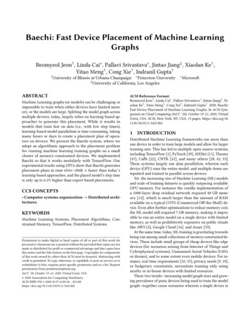
Baechi: Fast Device Placement of Machine Learning Graphs(a)(b)SoCC ’20, October 19–21, 2020, Virtual Event, USA(d)(c)(e)Figure 5: Operator Fusion Without Creating Cycles. When 𝑜𝑝𝑠𝑟𝑐 and 𝑜𝑝𝑑𝑠𝑡 are fused, some scenarios create a cycle (a),while others do not (b, c, d, e). Baechi fuses operators in a subset of “safe” cases, particularly (d, e).i) Operator Fusion: Fusing operators that are directly connected and in the same co-placement group; andii) Forward-Operator-Based Placement: Placing operators byonly considering the forward operators.Operator Fusion. Baechi fuses operators using either thecolocation constraints (Section 3.1) or co-placement optimizations (Section 3.2). This is new and different from TensorFlow’s fusion of operations. One challenge that appearshere is that this may introduce cycles in the graph, violatingthe DAG required by our algorithms.Figure 4 shows an example resulting from Figure 2—acycle is created when Step and UpdateStep are fused into anew meta-operator, and Weight and ApplyGrad are fused.Consider two nodes–source and destination–with an edgefrom source to destination. Merging source and destinationcreates a cycle if and only if there is at least one additionalpath from source to destination, other than the direct edge.Note that there cannot be a reverse destination to sourcepath as this means the original graph would have had acycle. In Figure 5a, fusing opsrc and opdst creates a cycle.Unfortunately, we found that pre-checking existence of suchadditional paths before fusing two operators is unscalable,because the model graph is massive.Instead, Baechi realizes that a necessary condition for anadditional path to exist is that the source has an out-degreeat least 2 and the destination has an in-degree at least 2(otherwise there wouldn’t be additional paths). Thus Baechiuses a conservative approach wherein it fuses two operatorsonly if the negation is true, i.e., either the source has an outdegree of at most 1, or the destination has an in-degree of atmost 1 (Figures 5d, 5e). This fusion rule misses a few fusions(Figures 5b, 5c) but it catches common patterns we observed,like Figure 5d.Forward-Operator-Based Placement. When memory issufficient (i.e., one device could run the entire model), Baechiconsiders only forward operators for placement and thereafter co-places each corresponding backward (gradient) operators on the same respective device as their forward counterparts. This is a commonly-used technique [2, 35]. This(a)(b)Figure 6: Operator Fusion. Avoiding Data Transfer Example. (a) Before Fusion. (b) After Fusion.significantly cuts placement time. When device memory isinsufficient, Baechi runs the placement algorithms usingboth forward and backward operators, forcing corresponding pairs to be co-placed using the heuristic of Section 3.2.Example: Benefits of Fusion. Figure 6a shows the placement of a subgraph of Figure 2 on two devices. Baechi firstplaces Grad on device-1. Baechi places the next operator,Step on the idle device-2, and colocates (due to TF constraints) UpdateStep on device-2. This creates communication between the devices. Assuming operators’ c

for running machine learning training graphs on a small cluster of memory-constrained devices. We implemented Baechi so that it works modularly with TensorFlow. Our experimental results using GPUs show that Baechi generates placement plans in time 654 -206K faster than today's learning-based approaches, and the placed model's step time