Transcription
Fundamentals of Image rtmouth.edu/ farid
0. Mathematical Foundations . . . . . . . . . . . . . . . . . . . . . . . . . . . . . . . . . . . . . . . . . . . . . 30.1: Vectors0.2: Matrices0.3: Vector Spaces0.4: Basis0.5: Inner Products and Projections [*]0.6: Linear Transforms [*]1. Discrete-Time Signals and Systems . . . . . . . . . . . . . . . . . . . . . . . . . . . . . . . . . . . . 141.1: Discrete-Time Signals1.2: Discrete-Time Systems1.3: Linear Time-Invariant Systems2. Linear Time-Invariant Systems . . . . . . . . . . . . . . . . . . . . . . . . . . . . . . . . . . . . . . . . 172.1: Space: Convolution Sum2.2: Frequency: Fourier Transform3. Sampling: Continuous to Discrete (and back) . . . . . . . . . . . . . . . . . . . . . . . . . 293.1: Continuous to Discrete: Space3.2: Continuous to Discrete: Frequency3.3: Discrete to Continuous4. Digital Filter Design . . . . . . . . . . . . . . . . . . . . . . . . . . . . . . . . . . . . . . . . . . . . . . . . . . 344.1: Choosing a Frequency Response4.2: Frequency Sampling4.3: Least-Squares4.4: Weighted Least-Squares5. Photons to Pixels . . . . . . . . . . . . . . . . . . . . . . . . . . . . . . . . . . . . . . . . . . . . . . . . . . . . . 395.1: Pinhole Camera5.2: Lenses5.3: CCD6. Point-Wise Operations . . . . . . . . . . . . . . . . . . . . . . . . . . . . . . . . . . . . . . . . . . . . . . . . 436.1: Lookup Table6.2: Brightness/Contrast6.3: Gamma Correction6.4: Quantize/Threshold6.5: Histogram Equalize7. Linear Filtering . . . . . . . . . . . . . . . . . . . . . . . . . . . . . . . . . . . . . . . . . . . . . . . . . . . . . . . 477.1: Convolution7.2: Derivative Filters7.3: Steerable Filters7.4: Edge Detection7.5: Wiener Filter8. Non-Linear Filtering . . . . . . . . . . . . . . . . . . . . . . . . . . . . . . . . . . . . . . . . . . . . . . . . . . 608.1: Median Filter8.2: Dithering9. Multi-Scale Transforms [*] . . . . . . . . . . . . . . . . . . . . . . . . . . . . . . . . . . . . . . . . . . . . 6310. Motion Estimation . . . . . . . . . . . . . . . . . . . . . . . . . . . . . . . . . . . . . . . . . . . . . . . . . . . 6410.1: Differential Motion10.2: Differential Stereo11. Useful Tools . . . . . . . . . . . . . . . . . . . . . . . . . . . . . . . . . . . . . . . . . . . . . . . . . . . . . . . . . 6911.1: Expectation/Maximization11.2: Principal Component Analysis [*]11.3: Independent Component Analysis [*][*] In progress
0. Mathematical Foundations0.1 Vectors0.1 Vectors0.2 MatricesFrom the preface of Linear Algebra and its Applications:0.3 Vector Spaces“Linear algebra is a fantastic subject. On the one handit is clean and beautiful.” – Gilbert Strang0.4 BasisThis wonderful branch of mathematics is both beautiful and useful. It is the cornerstone upon which signal and image processingis built. This short chapter can not be a comprehensive surveyof linear algebra; it is meant only as a brief introduction and review. The ideas and presentation order are modeled after Strang’shighly recommended Linear Algebra and its Applications.At the heart of linear algebra is machinery for solving linear equations. In the simplest case, the number of unknowns equals thenumber of equations. For example, here are a two equations intwo unknowns:0.5 Inner ProductsandProjections0.6 Linear Transformsy2x y 1(x,y) (2,3)2x y 1x y 5.(1)There are at least two ways in which we can think of solving theseequations for x and y. The first is to consider each equation asdescribing a line, with the solution being at the intersection of thelines: in this case the point (2, 3), Figure 0.1. This solution istermed a “row” solution because the equations are considered inisolation of one another. This is in contrast to a “column” solutionin which the equations are rewritten in vector form:xx y 5Figure 0.1 “Row” solution(1,5)( 3,3)(4,2)21 x 11 y 15 .(2)( 1,1)The solution reduces to finding values for x and y that scale thevectors (2, 1) and ( 1, 1) so that their sum is equal to the vector(1, 5), Figure 0.2. Of course the solution is again x 2 and y 3.These solutions generalize to higher dimensions. Here is an example with n 3 unknowns and equations:2u v w 54u 6v 0w 2 2u 7v 2w 9.3(3)(2,1)Figure 0.2 “Column”solution
Each equation now corresponds to a plane, and the row solutioncorresponds to the intersection of the planes (i.e., the intersectionof two planes is a line, and that line intersects the third plane ata point: in this case, the point u 1, v 1, w 2). In vectorform, the equations take the form:2115 4 u 6 v 0 w 2 . 2729 (4)The solution again amounts to finding values for u, v, and w thatscale the vectors on the left so that their sum is equal to the vectoron the right, Figure 0.3.(5, 2,9)Figure 0.3 “Column”solutionIn the context of solving linear equations we have introduced thenotion of a vector, scalar multiplication of a vector, and vectorsum. In its most general form, a n-dimensional column vector isrepresented as:x1 x2 x . , . (5)xnand a n-dimensional row vector as: y ( y1y2.yn ) .(6)Scalar multiplication of a vector x by a scalar value c, scales thelength of the vector by an amount c (Figure 0.2) and is given by:cv1 . c v . .cvn (7)The vector sum w x y is computed via the parallelogramconstruction or by “stacking” the vectors head to tail (Figure 0.2)and is computed by a pairwise addition of the individual vectorcomponents:x1 y 1w1 w2 x2 y 2 . . . .wnxn yn (8)The linear combination of vectors by vector addition and scalarmultiplication is one of the central ideas in linear algebra (moreon this later).4
0.2 MatricesIn solving n linear equations in n unknowns there are three quantities to consider. For example consider again the following set ofequations:2u v w 54u 6v 0w 2(9) 2u 7v 2w 9.On the right is the column vector:5 2 ,9 (10)and on the left are the three unknowns that can also be writtenas a column vector:u v .w (11)The set of nine coefficients (3 rows, 3 columns) can be written inmatrix form:21 1 4 6 0 2 7 2 (12)Matrices, like vectors, can be added and scalar multiplied. Notsurprising, since we may think of a vector as a skinny matrix: amatrix with only one column. Consider the following 3 3 matrix:a1 a4A a7 a2a5a8a3a6 .a9 (13)The matrix cA, where c is a scalar value, is given by:ca1cA ca4ca7 ca2ca5ca8ca3ca6 .ca9 (14)And the sum of two matrices, A B C, is given by:a1 a4a7 a2a5a8a3b1 c1a6 b4 c4a9b7 c7 5b2 c2b5 c5b8 c8b3 c3b6 c6 .b9 c9 (15)
With the vector and matrix notation we can rewrite the threeequations in the more compact form of A x b:2 4 2 1 1u5 6 0v 2 .7 2w9 (16)Where the multiplication of the matrix A with vector x must besuch that the three original equations are reproduced. The firstcomponent of the product comes from “multiplying” the first rowof A (a row vector) with the column vector x as follows:(2 1u 1 ) v ( 2u 1v 1w ) .w (17)This quantity is equal to 5, the first component of b, and is simplythe first of the three original equations. The full product is computed by multiplying each row of the matrix A with the vector xas follows:52u 1v 1w21 1u 4 4u 6v 0w 6 0v 2 .9 2u 7v 2w 2 7 2w (18)In its most general form the product of a m n matrix with an dimensional column vector is a m dimensional column vectorwhose ith component is:nXaij xj ,(19)j 1where aij is the matrix component in the ith row and j th column.The sum along the ith row of the matrix is referred to as the innerproduct or dot product between the matrix row (itself a vector) andthe column vector x. Inner products are another central idea inlinear algebra (more on this later). The computation for multiplying two matrices extends naturally from that of multiplying amatrix and a vector. Consider for example the following 3 4 and4 2 matrices:a11A a21a31 a12a22a32a13a23a33b11 b21and B b31b41 a14a24 a34 The product C AB is a 3 2 matrix given by:a11 b11 a12 b21 a13 b31 a14 b41a21 b11 a22 b21 a23 b31 a24 b41a31 b11 a32 b21 a33 b31 a34 b41b12b22 .b32 b42 a11 b12 a12 b22 a13 b32 a14 b42a21 b12 a22 b22 a23 b32 a24 b42a31 b12 a32 b22 a33 b32 a34 b426(20)!.(21)
That is, the i, j component of the product C is computed froman inner product of the ith row of matrix A and the j th columnof matrix B. Notice that this definition is completely consistentwith the product of a matrix and vector. In order to multiplytwo matrices A and B (or a matrix and a vector), the columndimension of A must equal the row dimension of B. In other wordsif A is of size m n, then B must be of size n p (the product isof size m p). This constraint immediately suggests that matrixmultiplication is not commutative: usually AB 6 BA. Howevermatrix multiplication is both associative (AB)C A(BC) anddistributive A(B C) AB AC.The identity matrix I is a special matrix with 1 on the diagonaland zero elsewhere:I1 0 0 1 . .0 0 .0 00 0 . . 0 1 (22)Given the definition of matrix multiplication, it is easily seen thatfor any vector x, I x x, and for any suitably sized matrix, IA Aand BI B.In the context of solving linear equations we have introduced thenotion of a vector and a matrix. The result is a compact notationfor representing linear equations, A x b. Multiplying both sidesby the matrix inverse A 1 yields the desired solution to the linearequations:A 1 A x A 1 bI x A 1 b x A 1 b(23)A matrix A is invertible if there exists 1 a matrix B such thatBA I and AB I, where I is the identity matrix. The matrix B is the inverse of A and is denoted as A 1 . Note that thiscommutative property limits the discussion of matrix inverses tosquare matrices.Not all matrices have inverses. Let’s consider some simple examples. The inverse of a 1 1 matrix A ( a ) is A 1 ( 1/a );but the inverse does not exist when a 0. The inverse of a 2 21The inverse of a matrix is unique: assume that B and C are both theinverse of matrix A, then by definition B B(AC) (BA)C C, so that Bmust equal C.7
matrix can be calculated as: acbd 1 1ad bc d b c a ,(24)but does not exist when ad bc 0. Any diagonal matrix isinvertible: A a1. .an 1/a1.and A 1 .1/an , (25)as long as all the diagonal components are non-zero. The inverseof a product of matrices AB is (AB) 1 B 1 A 1 . This is easilyproved using the associativity of matrix multiplication. 2 Theinverse of an arbitrary matrix, if it exists, can itself be calculatedby solving a collection of linear equations. Consider for example a3 3 matrix A whose inverse we know must satisfy the constraintthat AA 1 I:2 4 2 1 1 6 0 x17 2 x3 e1 x2 e21 0 0 e3 0 1 0 .(26)0 0 1 This matrix equation can be considered “a column at a time”yielding a system of three equations Ax 1 e 1 , Ax 2 e 2 , andAx 3 e 3 . These can be solved independently for the columnsof the inverse matrix, or simultaneously using the Gauss-Jordanmethod.A system of linear equations A x b can be solved by simplyleft multiplying with the matrix inverse A 1 (if it exists). Wemust naturally wonder the fate of our solution if the matrix is notinvertible. The answer to this question is explored in the nextsection. But before moving forward we need one last definition.The transpose of a matrix A, denoted as At , is constructed byplacing the ith row of A into the ith column of At . For example:A 1 2 14 6 0 1and At 21 4 6 0 (27)In general, the transpose of a m n matrix is a n m matrix with(At )ij Aji . The transpose of a sum of two matrices is the sum of2In order to prove (AB) 1 B 1 A 1 , we must show (AB)(B 1 A 1 ) I: (AB)(B 1 A 1 ) A(BB 1 )A 1 AIA 1 AA 1 I, and that(B 1 A 1 )(AB) I: (B 1 A 1 )(AB) B 1 (A 1 A)B B 1 IB B 1 B I.8
the transposes: (A B)t At B t. The transpose of a product oftwo matrices has the familiar form (AB)t B t At . And the transpose of the inverse is the inverse of the transpose: (A 1 )t (At ) 1 .Of particular interest will be the class of symmetric matrices thatare equal to their own transpose At A. Symmetric matrices arenecessarily square, here is a 3 3 symmetric matrix:2 1 4A 1 6 0 ,4 0 3 (28)notice that, by definition, aij aji .0.3 Vector SpacesThe most common vector space is that defined over the reals, denoted as Rn . This space consists of all column vectors with nreal-valued components, with rules for vector addition and scalarmultiplication. A vector space has the property that the addition and multiplication of vectors always produces vectors that liewithin the vector space. In addition, a vector space must satisfythe following properties, for any vectors x, y, z, and scalar c:1.2.3.4.5.6.7.8. x y y x( x y) z x ( y z)there exists a unique “zero” vector 0 such that x 0 xthere exists a unique “inverse” vector x such that x ( x) 01 x x(c1 c2 ) x c1 (c2 x)c( x y ) c x c y(c1 c2 ) x c1 x c2 xVector spaces need not be finite dimensional, R is a vector space.Matrices can also make up a vector space. For example the spaceof 3 3 matrices can be thought of as R9 (imagine stringing outthe nine components of the matrix into a column vector).A subspace of a vector space is a non-empty subset of vectors thatis closed under vector addition and scalar multiplication. Thatis, the following constraints are satisfied: (1) the sum of any twovectors in the subspace remains in the subspace; (2) multiplicationof any vector by a scalar yields a vector in the subspace. Withthe closure property verified, the eight properties of a vector spaceautomatically hold for the subspace.Example 0.1Consider the set of all vectors in R2 whose com-ponents are greater than or equal to zero. The sum of any two9
vectors in this space remains in the space, but multiplication of, 1 1for example, the vectorby 1 yields the vector2 2which is no longer in the space. Therefore, this collection ofvectors does not form a vector space.Vector subspaces play a critical role in understanding systems oflinear equations of the form A x b. Consider for example thefollowing system:u1 u2u3v1 b1x1v2 b2 x2v3b3 (29)Unlike the earlier system of equations, this system is over-constrained,there are more equations (three) than unknowns (two). A solution to this system exists if the vector b lies in the subspace of thecolumns of matrix A. To see why this is so, we rewrite the abovesystem according to the rules of matrix multiplication yielding anequivalent form:u1v1b1 x1 u2 x2 v2b2 . u3v3b3 (30)In this form, we see that a solution exists when the scaled columnsof the matrix sum to the vector b. This is simply the closureproperty necessary for a vector subspace.The vector subspace spanned by the columns of the matrix A iscalled the column space of A. It is said that a solution to A x bexists if and only if the vector b lies in the column space of A.Example 0.2Consider the following over-constrained system:152044x b!! A b1uv b2b3The column space of A is the plane spanned by the vectors( 1 5 2 )t and ( 0 4 4 )t . Therefore, the solution b can notbe an arbitrary vector in R3 , but is constrained to lie in theplane spanned by these two vectors.At this point we have seen three seemingly different classes oflinear equations of the form A x b, where the matrix A is either:1. square and invertible (non-singular),10
2. square but not invertible (singular),3. over-constrained.In each case solutions to the system exist if the vector b lies in thecolumn space of the matrix A. At one extreme is the invertiblen n square matrix whose solutions may be any vector in the wholeof Rn . At the other extreme is the zero matrix A 0 with onlythe zero vector in it’s column space, and hence the only possiblesolution. In between are the singular and over-constrained cases,where solutions lie in a subspace of the full vector space.The second important vector space is the nullspace of a matrix.The vectors that lie in the nullspace of a matrix consist of allsolutions to the system A x 0. The zero vector is always in thenullspace.Example 0.3Consider the following system:152044196A x!uvw! 0000The nullspace of A contains the zero vector ( u!vw )t ( 000 )t .Notice also that the third column of A is the sum of the first twocolumns, therefore the nullspace of A also contains all vectors ofthe form ( uvw )t ( cc c )t (i.e., all vectors lying on a3one-dimensional line in R ).0.4 Basis(2,2)Recall that if the matrix A in the system A x b is invertible, thenleft multiplying with A 1 yields the desired solution: x A 1 b.In general it is said that a n n matrix is invertible if it has rankn or is full rank, where the rank of a matrix is the number oflinearly independent rows in the matrix. Formally, a set of vectors u1 , u2 , ., un are linearly independent if:c1 u1 c2 u2 . cn un 0(31)is true only when c1 c2 . cn 0. Otherwise, the vectorsare linearly dependent. In other words, a set of vectors are linearlydependent if at least one of the vectors can be expressed as a sumof scaled copies of the remaining vectors.Linear independence is easy to visualize in lower-dimensional subspaces. In 2-D, two vectors are linearly dependent if they lie alonga line, Figure 0.4. That is, there is a non-trivial combination of the( 1, 1)(2,2)( 2,0)( 1,2)(2,2)( 2,0)Figure 0.4 Linearly dependent11(top/bottom) and independent (middle).
vectors that yields the zero vector. In 2-D, any three vectors areguaranteed to be linearly dependent. For example, in Figure 0.4,the vector ( 1 2 ) can be expressed as a sum of the remaininglinearly independent vectors: 23 ( 2 0 ) ( 2 2 ). In 3-D, threevectors are linearly dependent if they lie in the same plane. Alsoin 3-D, any four vectors are guaranteed to be linearly dependent.Linear independence is directly related to the nullspace of a matrix. Specifically, the columns of a matrix are linearly independent(i.e., the matrix is full rank) if the matrix nullspace contains onlythe zero vector. For example, consider the following system oflinear equations:u1 u2u3 v1v2v3w1x10 w2x2 0 .w3x30 (32)Recall that the nullspace contains all vectors x such that x1 u x2 v x3 w 0. Notice that this is also the condition for linearindependence. If the only solution is the zero vector then thevectors are linearly independent and the matrix is full rank andinvertible.Linear independence is also related to the column space of a matrix. If the column space of a n n matrix is all of Rn , then thematrix is full rank. For example, consider the following system oflinear equations:u1 u2u3 v1v2v3w1x1b1w2 x2 b2 .w3x3b3 (33)If the the matrix is full rank, then the solution b can be any vectorin R3 . In such cases, the vectors u, v , w are said to span the space.Now, a linear basis of a vector space is a set of linearly independentvectors that span the space. Both conditions are important. Givenan n dimensional vector space with n basis vectors v1 , ., vn , anyvector u in the space can be written as a linear combination ofthese n vectors: u a1 v 1 . an v n .(34)In addition, the linear independence guarantees that this linearcombination is unique. If there is another combination such that: u b1 v 1 . bn v n ,12(35)
then the difference of these two representations yields 0 (a1 b1 )v 1 . (an bn )v n c1 v 1 . cn v n(36)which would violate the linear independence condition. Whilethe representation is unique, the basis is not. A vector space hasinfinitely many different bases. For example in R2 any two vectorsthat do not lie on a line form a basis, and in R3 any three vectorsthat do not lie in a common plane or line form a basis.Example 0.4The vectors ( 10 ) and ( 01 ) form the canonicalbasis for R2 . These vectors are both linearly independent andspan the entire vector space.Example 0.5The vectors ( 100 ), ( 010 ) and ( 100)do not form a basis for R3 . These vectors lie in a 2-D plane anddo not span the entire vector space.Example 0.6and ( 1The vectors ( 1 100 ), ( 0 10 ), ( 002 ),0 ) do not form a basis. Although these vectorsspan the vector space, the fourth vector is linearly dependent onthe first two. Removing the fourth vector leaves a basis for R3 .0.5 Inner Products and Projections0.6 Linear Transforms13
1. Discrete-Time Signals and Systems1.1 Discrete-Time Signals1.1 Discrete-TimeSignalsA discrete-time signal is represented as a sequence of numbers, f ,where the xth number in the sequence is denoted as f [x]:1.2 Discrete-TimeSystemsf1.3 Linear TimeInvariant Systemsf[x] x ,(1.1)where x is an integer. Note that from this definition, a discretetime signal is defined only for integer values of x. For example,the finite-length sequence shown in Figure 1.1 is represented bythe following sequence of numbersf { f [1] {0xFigure 1.1 {f [x]},1f [2] .2 4 8f [12] }7 65 4 32 1 }.(1.2)For notational convenience, we will often drop the cumbersomenotation of Equation (1.1), and refer to the entire sequence simply as f [x]. Discrete-time signals often arise from the periodicsampling of continuous-time (analog) signals, a process that wewill cover fully in later chapters.Discrete-time signal1.2 Discrete-Time Systemsf[x]Tg[x]In its most general form, a discrete-time system is a transformationthat maps a discrete-time signal, f [x], onto a unique g[x], and isdenoted as:g[x] T {f [x]}Figure 1.2Discrete-time systemExample 1.1(1.3)Consider the following system:g[x] NX1f [x k].2N 1k NIn this system, the ith number in the output sequence is computed as the average of 2N 1 elements centered around the ithf[x]input element. As shown in Figure 1.3, with N 2, the outputvalue at x 5 is computed as 1/5 times the sum of the five inputx357Figure 1.3 MovingerageAv-elements between the dotted lines. Subsequent output values arecomputed by sliding these lines to the right.Although in the above example, the output at each position depended on only a small number of input values, in general, thismay not be the case, and the output may be a function of all inputvalues.14
1.3 Linear Time-Invariant SystemsOf particular interest to us will be a class of discrete-time systemsthat are both linear and time-invariant. A system is said to belinear if it obeys the rules of superposition, namely:T {af1 [x] bf2 [x]} aT {f1 [x]} bT {f2 [x]},(1.4)for any constants a and b. A system, T {·} that maps f [x] onto g[x]is shift- or time-invariant if a shift in the input causes a similarshift in the output:g[x] T {f [x]}Example 1.2 g[x x0 ] T {f [x x0 ]}.(1.5)Consider the following system:g[x] f [x] f [x 1], x .In this system, the kth number in the output sequence is computed as the difference between the kth and kth-1 elements inthe input sequence. Is this system linear? We need only showthat this system obeys the principle of superposition:T {af1 [x] bf2 [x]} (af1 [x] bf2 [x]) (af1 [x 1] bf2 [x 1]) (af1 [x] af1 [x 1]) (bf2 [x] bf2 [x 1]) a(f1 [x] f1 [x 1]) b(f2 [x] f2 [x 1])which, according to Equation (1.4), makes T {·} linear. Is thissystem time-invariant? First, consider the shifted signal, f1 [x] f [x x0 ], then:g1 [x] f1 [x] f1 [x 1] f [x x0 ] f [x 1 x0 ],and,g[x x0 ] f [x x0 ] f [x 1 x0 ] g1 [x],so that this system is time-invariant.Example 1.3Consider the following system:g[x] f [nx], x ,where n is a positive integer. This system creates an outputsequence by selecting every nth element of the input sequence.Is this system linear?T {af1 [x] bf2 [x]} af1 [nx] bf2 [nx]which, according to Equation (1.4), makes T {·} linear. Is thissystem time-invariant? First, consider the shifted signal, f1 [x] f [x x0 ], then:g1 [x] f1 [nx] f [nx x0 ],but,g[x x0 ] f [n(x x0 )] 6 g1 [x],so that this system is not time-invariant.15f[x]xg[x]xFigure 1.4 Backwarddifference
The precise reason why we are particularly interested in lineartime-invariant systems will become clear in subsequent chapters.But before pressing on, the concept of discrete-time systems isreformulated within a linear-algebraic framework. In order to accomplish this, it is necessary to first restrict ourselves to considerinput signals of finite length. Then, any discrete-time linear system can be represented as a matrix operation of the form: g M f ,(1.6)where, f is the input signal, g is the output signal, and the matrixM embodies the discrete-time linear system.Example 1.4Consider the following system:g[x] f [x 1],1 x 8.The output of this system is a shifted copy of the input signal,and can be formulated in matrix notation as:g[1] g[2] g[3] g[4] g[5] g[6] g[7]g[8] 0 1 0 0 0 0 00 0010000000010000000010000000010000000010000000011f [1]0 f [2] 0 f [3] f [4] 0 0 f [5] 0 f [6] f [7]0f [8]0 Note that according to the initial definition of the system, theoutput signal at x 1 is undefined (i.e., g[1] f [0]). In theabove matrix formulation we have adopted a common solutionto this problem by considering the signal as wrapping arounditself and setting g[1] f [8].Any system expressed in the matrix notation of Equation (1.6) isa discrete-time linear system, but not necessarily a time-invariantsystem. But, if we constrain ourselves to Toeplitz matrices, thenthe resulting expression will be a linear time-invariant system. AToeplitz matrix is one in which each row contains a shifted copyof the previous row. For example, a 5 5 Toeplitz matrix is of theformM m1 m 5 m4 m3m2m2m1m5m4m3m3m2m1m5m4m4m3m2m1m5 m5m4 m3 m2 m1(1.7)It is important to feel comfortable with this formulation becauselater concepts will be built upon this linear algebraic framework.16
2. Linear Time-Invariant SystemsOur interest in the class of linear time-invariant systems (LTI) ismotivated by the fact that these systems have a particularly convenient and elegant representation, and this representation leadsus to several fundamental tools in signal and image processing.2.1 Space: Convolution SumIn the previous section, a discrete-time signal was represented asa sequence of numbers. More formally, this representation is interms of the discrete-time unit impulse defined as:(δ[x] Xk (2.1)f [k]δ[x k],(2.2)where the shifted impulse δ[x k] 1 when x k, and is zeroelsewhere.Example 2.1Consider the following discrete-time signal, centered at x 0.f [x] (.002 1400.),this signal can be expressed as a sum of scaled and shifted unitimpulses:f [x] 2δ[x 1] 1δ[x] 4δ[x 1] f [ 1]δ[x 1] f [0]δ[x] f [1]δ[x 1] 1Xf [k]δ[x k].k 1Let’s now consider what happens when we present a linear timeinvariant system with this new representation of a discrete-timesignal:g[x] T {f [x]} T X k 172.2 Frequency:Fourier Transform1x1, x 00, x 6 0.Any discrete-time signal can be represented as a sum of scaled andshifted unit-impulses:f [x] 2.1 Space: Convolution Sum f [k]δ[x k] . (2.3)Figure 2.1 Unit impulse
By the property of linearity, Equation (1.4), the above expressionmay be rewritten as:g[x] Xk f [k]T {δ[x k]}.(2.4)Imposing the property of time-invariance, Equation (1.5), if h[x] isthe response to the unit-impulse, δ[x], then the response to δ[x k]is simply h[x k]. And now, the above expression can be rewrittenas: Xg[x] k f [k]h[x k].(2.5)Consider for a moment the implications of the above equation.The unit-impulse response, h[x] T {δ[x]}, of a linear time-invariantsystem fully characterizes that system. More precisely, given theunit-impulse response, h[x], the output, g[x], can be determinedfor any input, f [x].The sum in Equation (2.5) is commonly called the convolutionsum and may be expressed more compactly as:g[x] f [x] h[x].(2.6)A more mathematically correct notation is (f h)[x], but for laternotational considerations, we will adopt the above notation.Example 2.2response:Consider the following finite-length unit-impulseh[x]h[x]0f[x] ( 24 2 ) ,and the input signal, f [x], shown in Figure 2.2. Then the outputsignal at, for example, x 2, is computed as:g[ 2] 0 1Xf [k]h[ 2 k]k 3 f [ 3]h[1] f [ 2]h[0] f [ 1]h[ 1].g[ 2]Figure 2.2 Convolution:g[x] f [x] h[x]The next output sum at x 1, is computed by “sliding” theunit-impulse response along the input signal and computing asimilar sum.Since linear time-invariant systems are fully characterized by convolution with the unit-impulse response, properties of such systems can be determined by considering properties of the convolution operator. For example, convolution is commutative:f [x] h[x] Xk f [k]h[x k],18let j x k
X j f [x j]h[j] h[x] f [x]. Xj h[j]f [x j](2.7)Convolution also distributes over addition: Xf [x] (h1 [x] h2 [x]) k X k X k f [k](h1 [x k] h2 [x k])f [k]h1 [x k] f [k]h2 [x k]f [k]h1 [x k] Xk f [k]h2 [x k] f [x] h1 [x] f [x] h2 [x].(2.8)A final useful property of linear time-invariant systems is thata cascade of systems can be combined into a single system withimpulse response equal to the convolution of the individual impulseresponses. For example, for a cascade of two systems:f[x]f[x](f [x] h1 [x]) h2 [x] f [x] (h1 [x] h2 [x]).(2.9)This property is fairly straight-forward to prove, and offers a goodexercise in manipulating the convolution sum:g1 [x] f [x] h1 [x] Xk f [k]h1 [x k] and,(2.10)g2 [x] (f [x] h1 [x]) h2 [x] g1 [x] h2 [x] Xj Xj Xk Xk g1 [j]h2 [x j] substituting for g1 [x], Xk f [k] f [k] f
it is clean and beautiful." - Gilbert Strang This wonderful branch of mathematics is both beautiful and use-ful. It is the cornerstone upon which signal and image processing is built. This short chapter can not be a comprehensive survey of linear algebra; it is meant only as a brief introduction and re-view.