Transcription
Convex Optimization OverviewStephen Boyd Steven Diamond Enzo BussetiAkshay Agrawal Junzi ZhangEE & CS DepartmentsStanford University1
OutlineMathematical OptimizationConvex OptimizationSolvers & Modeling LanguagesExamplesSummary2
OutlineMathematical OptimizationConvex OptimizationSolvers & Modeling LanguagesExamplesSummaryMathematical Optimization3
Optimization problemminimize f0 (x)subject to fi (x) 0, i 1, . . . , mgi (x) 0, i 1, . . . , pI x Rn is (vector) variable to be chosenI f0 is the objective function, to be minimizedI f1 , . . . , fm are the inequality constraint functionsI g1 , . . . , gp are the equality constraint functionsI variations: maximize objective, multiple objectives, . . .Mathematical Optimization4
Finding good (or best) actionsI x represents some action, e.g.,IIIIItrades in a portfolioairplane control surface deflectionsschedule or assignmentresource allocationtransmitted signalI constraints limit actions or impose conditions on outcomeI the smaller the objective f0 (x), the betterIIIItotal cost (or negative profit)deviation from desired or target outcomefuel useriskMathematical Optimization5
Engineering designI x represents a design (of a circuit, device, structure, . . . )I constraints come fromI manufacturing processI performance requirementsI objective f0 (x) is combination of cost, weight, power, . . .Mathematical Optimization6
Finding good modelsI x represents the parameters in a modelI constraints impose requirements on model parameters(e.g., nonnegativity)I objective f0 (x) is the prediction error on some observed data(and possibly a term that penalizes model complexity)Mathematical Optimization7
InversionI x is something we want to estimate/reconstruct, givensome measurement yI constraints come from prior knowledge about xI objective f0 (x) measures deviation between predicted andactual measurementsMathematical Optimization8
Worst-case analysis (pessimization)I variables are actions or parameters out of our control(and possibly under the control of an adversary)I constraints limit the possible values of the parametersI minimizing f0 (x) finds worst possible parameter valuesI if the worst possible value of f0 (x) is tolerable, you’re OKI it’s good to know what the worst possible scenario can beMathematical Optimization9
Optimization-based modelsI model an entity as taking actions that solve an optimizationproblemIIIIan individual makes choices that maximize expected utilityan organism acts to maximize its reproductive successreaction rates in a cell maximize growthcurrents in an electric circuit minimize total powerMathematical Optimization10
Optimization-based modelsI model an entity as taking actions that solve an optimizationproblemIIIIan individual makes choices that maximize expected utilityan organism acts to maximize its reproductive successreaction rates in a cell maximize growthcurrents in an electric circuit minimize total powerI (except the last) these are very crude modelsI and yet, they often work very wellMathematical Optimization10
SummaryI summary: optimization arises everywhereMathematical Optimization11
SummaryI summary: optimization arises everywhereI the bad news: most optimization problems are intractablei.e., we cannot solve themMathematical Optimization11
SummaryI summary: optimization arises everywhereI the bad news: most optimization problems are intractablei.e., we cannot solve themI an exception: convex optimization problems are tractablei.e., we (generally) can solve themMathematical Optimization11
OutlineMathematical OptimizationConvex OptimizationSolvers & Modeling LanguagesExamplesSummaryConvex Optimization12
Convex optimization problemconvex optimization problem:minimize f0 (x)subject to fi (x) 0,Ax bi 1, . . . , mI variable x RnI equality constraints are linearI f0 , . . . , fm are convex: for θ [0, 1],fi (θx (1 θ)y ) θfi (x) (1 θ)fi (y )i.e., fi have nonnegative (upward) curvatureConvex Optimization13
WhyI beautiful, nearly complete theoryI duality, optimality conditions, . . .Convex Optimization14
WhyI beautiful, nearly complete theoryI duality, optimality conditions, . . .I effective algorithms, methods (in theory and practice)I get global solution (and optimality certificate)I polynomial complexityConvex Optimization14
WhyI beautiful, nearly complete theoryI duality, optimality conditions, . . .I effective algorithms, methods (in theory and practice)I get global solution (and optimality certificate)I polynomial complexityI conceptual unification of many methodsConvex Optimization14
WhyI beautiful, nearly complete theoryI duality, optimality conditions, . . .I effective algorithms, methods (in theory and practice)I get global solution (and optimality certificate)I polynomial complexityI conceptual unification of many methodsI lots of applications (many more than previously thought)Convex Optimization14
Application areasI machine learning, statisticsI financeI supply chain, revenue management, advertisingI controlI signal and image processing, visionI networkingI circuit designI combinatorial optimizationI quantum mechanicsI flux-based analysisConvex Optimization15
The approachI try to formulate your optimization problem as convexI if you succeed, you can (usually) solve it (numerically)I using generic software if your problem is not really bigI by developing your own software otherwiseConvex Optimization16
The approachI try to formulate your optimization problem as convexI if you succeed, you can (usually) solve it (numerically)I using generic software if your problem is not really bigI by developing your own software otherwiseI some tricks:I change of variablesI approximation of true objective, constraintsI relaxation: ignore terms or constraints you can’t handleConvex Optimization16
OutlineMathematical OptimizationConvex OptimizationSolvers & Modeling LanguagesExamplesSummarySolvers & Modeling Languages17
Medium-scale solversI 1000s–10000s variables, constraintsI reliably solved by interior-point methods on single machine(especially for problems in standard cone form)I exploit problem sparsityI not quite a technology, but getting thereI used in control, finance, engineering design, . . .Solvers & Modeling Languages18
Large-scale solversI 100k – 1B variables, constraintsI solved using custom (often problem specific) methodsIIIIlimited memory BFGSstochastic subgradientblock coordinate descentoperator splitting methodsI require custom implementation, tuning for each problemI used in machine learning, image processing, . . .Solvers & Modeling Languages19
Modeling languagesI (new) high level language support for convex optimizationI describe problem in high level languageI description automatically transformed to a standard formI solved by standard solver, transformed back to original formI implementations:IIIIYALMIP, CVX (Matlab)CVXPY (Python)Convex.jl (Julia)CVXR (R)Solvers & Modeling Languages20
CVX(Grant & Boyd, 2005)cvx beginvariable x(n)% declare vector variableminimize sum(square(A*x-b)) gamma*norm(x,1)subject to norm(x,inf) 1cvx endI A, b, gamma are constants (gamma nonnegative)I after cvx endI problem is converted to standard form and solvedI variable x is over-written with (numerical) solutionSolvers & Modeling Languages21
CVXPY(Diamond & Boyd, 2013); (Agrawal et al., 2018)import cvxpy as cpx cp.Variable(n)cost cp.sum squares(A@x-b) gamma*cp.norm(x,1)prob cp.Problem(cp.Minimize(cost),[cp.norm(x,"inf") 1])opt val prob.solve()solution x.valueI A, b, gamma are constants (gamma nonnegative)I solve method converts problem to standard form, solves,assigns value attributesSolvers & Modeling Languages22
Convex.jl(Udell et al., 2014)using Convexx Variable(n);cost sum squares(A*x-b) gamma*norm(x,1);prob minimize(cost, [norm(x,Inf) 1]);opt val solve!(prob);solution x.value;I A, b, gamma are constants (gamma nonnegative)I solve! method converts problem to standard form, solves,assigns value attributesSolvers & Modeling Languages23
Modeling languagesI enable rapid prototyping (for small and medium problems)I ideal for teaching (can do a lot with short scripts)I slower than custom methods, but often not muchI current work focuses on extension to large problemsSolvers & Modeling Languages24
OutlineMathematical OptimizationConvex OptimizationSolvers & Modeling LanguagesExamplesSummaryExamples25
Radiation treatment planningI radiation beams with intensities xj 0 directed at patientI radiation dose yi received in voxel iI y AxI A Rm n comes from beam geometry, physicsI goal is to choose x to deliver prescribed radiation dose diI di 0 for non-tumor voxelsI di 0 for tumor voxelsI y d not possible, so we’ll need to compromiseI typical problem has n 103 beams, m 106 voxelsExamples26
Radiation treatment planning via convex optimizationPminimizei fi (yi )subject to x 0, y AxI variables x Rn , y RmI objective terms arefi (yi ) wiover (yi di ) wiunder (di yi ) I wiover and wiunder are positive weightsI i.e., we charge linearly for over- and under-dosingI a convex problemExamples27
ExampleI real patient case with n 360 beams, m 360000 voxelsI optimization-based plan essentially the same as plan usedExamples28
ExampleI real patient case with n 360 beams, m 360000 voxelsI optimization-based plan essentially the same as plan usedI but we computed the plan in a few seconds on a GPUI original plan took hours of least-squares weight tweakingExamples28
Image in-paintingI guess pixel values in obscured/corrupted parts of imageI total variation in-painting: choose pixel values xij R3 tominimize total variationX xi 1,j xij TV(x) xi,j 1 xij2i,jI a convex problemExamples29
Example512 512 grayscale image (n 300000 variables)Examples30
ExampleExamples31
Example512 512 color image (n 800000), 80% of pixels removedExamples32
Example80% of pixels removedExamples33
ControlPT 1minimizet 0 (xt , ut ) T (xT )subject to xt 1 Axt But(xt , ut ) C, xT CTI variables areI system states x1 , . . . , xT RnI inputs or actions u0 , . . . , uT 1 RmI is stage cost, T is terminal costI C is state/action constraints; CT is terminal constraintI convex problem when costs, constraints are convexI applications in many fieldsExamples34
ExampleI n 8 states, m 2 inputs, horizon T 50I randomly chosen A, B (with A I )I input constraint kut k 1I terminal constraint xT 0 (‘regulator’)I (x, u) kxk22 kuk22 (traditional)I random initial state x0Examples35
ExampleExamples36
Support vector machine classifier with 1 -regularizationI given data (xi , yi ), i 1, . . . , mI xi Rn are feature vectorsI y { 1} are associated boolean outcomesI linear classifier ŷ sign(β T x v )I find parameters β, v by minimizing (convex function) X (1/m)1 yi (β T xi v ) λkβk1i I first term is average hinge lossI second term shrinks coefficients in β and encourages sparsityI λ 0 is (regularization) parameterI simultaneously selects features and fits classifierExamples37
ExampleI n 20 featuresI trained and tested on m 1000 examples eachExamples38
Exampleβi vs. λ (regularization path)Examples39
OutlineMathematical OptimizationConvex OptimizationSolvers & Modeling LanguagesExamplesSummarySummary40
SummaryI convex optimization problems arise in many applicationsI convex optimization problems can be solved effectivelyI using generic methods for not huge problemsI by developing custom methods for huge problemsI high level language support(CVX/CVXPY/Convex.jl/CVXR) makes prototyping easySummary41
Resourcesmany researchers have worked on the topics coveredI Convex Optimization (book)I EE364a (course slides, videos, code, homework, . . . )I software CVX, CVXPY, Convex.jl, CVXRall available onlineSummary42
Optimization-based models I model an entity as taking actions that solve an optimization problem I an individual makes choices that maximize expected utility I an organism acts to maximize its reproductive success I reaction rates in a cell maximize growth I currents in an electric circuit minimize total power I (except the last) these are very crude models I and yet, they often work very well