Transcription
3 445b 0287840 LEsmand G. NgBarry w. Peyton.-.-. .
ORNL/TM-11960Engineering Physics and Mathematics DivisionMathematical Sciences SectionBLOCK SPARSE CHOLESKY ALGORITHMS O NADVANCED UNIPROCESSOR COMPUTERSEsmond G. NgBarry W. PeytonMathematical Sciences SectionOak Ridge National LaboratoryP.O. Box 2008, Bldg. 6012Oak Ridge, T N 37831-6367DATE PUBLISHED-DECEMBER 1 9 9 1Research was supported by the Applied Mathematical Sciences Research Program of the Office of Energy Research,U.S. Department of Energy.Prepared by theOak Ridge National LaboratoryOak Ridge, Tennessee 37831managed byMartin Marietta Energy Systems, Inc.for theU.S. DEPARTMENT OF ENERGYunder Contract No. DE-AC05-S40R21400 1 3 4456 0287890 Z
Contents1 Introduction . . . . . . . . . . . . . . . . . . . . . . . . . . . . . . . . . . . . .2 Background material . . . . . . . . . . . . . . . . . . . . . . . . . . . . . . . .2.1 Column-based Cholesky factorization methods . . . . . . . . . . . . . .2.2 Supernodes and elimination trees . . . . . . . . . . . . . . . . . . . . . .2.3 Supernode-based Cholesky algorithms: previous work . . . . . . . . . .2.3.1 Left-looking sup-col Cholesky factorization . . . . . . . . . . . .2.3.2 Multifrontal Cholesky factorization . . . . . . . . . . . . . . . . .3 Left-looking sup-sup Cholesky factorization . . . . . . . . . . . . . . . . . . .4 Implementation details and options . . . . . . . . . . . . . . . . . . . . . . . .4.1 Reuse of d a t a in cache . . . . . . . . . . . . . . . . . . . . . . . . . . . .4.2 Traversing row-structure sets . . . . . . . . . . . . . . . . . . . . . . . .4.3 Enhancements to the multifrontal method . . . . . . . . . . . . . . . . .4.4 Refinements for left-looking sup-col and sup-sup Cholesky . . . . . . .5 Performance results . . . . . . . . . . . . . . . . . . . . . . . . . . . . . . . . .5.1 IBMRS/6000 . . . . . . . . . . . . . . . . . . . . . . . . . . . . . . . . .5.2 DEC5OOO . . . . . . . . . . . . . . . . . . . . . . . . . . . . . . . . . . .5.3 Stardent P3000 (without vectorization) . . . . . . . . . . . . . . . . . .5.4 Stardent P3000 (with vectorization) . . . . . . . . . . . . . . . . . . . .5.5 CrayY-MP . . . . . . . . . . . . . . . . . . . . . . . . . . . . . . . . . .5.6 Work storage requirements . . . . . . . . . . . . . . . . . . . . . . . . .6 Concluding remarks . . . . . . . . . . . . . . . . . . . . . . . . . . . . . . . .7 References . . . . . . . . . . . . . . . . . . . . . . . . . . . . . . . . . . . . . .1225589111212131415161921222223242426
BLOCK SPARSE CHOLESKY ALGORITHMS O NADVANCED UNIPROCESSOR COMPUTERSEsmond G. NgBarry W. PeytonAbstractAs with many other linear algebra algorithms, devising a portable iniplementation of sparse Cholesky factorization that performs well on the broad range ofcomputer architectures currently available is a formidable challenge. Even afterlimiting our attention to machines with only one processor, as we have done in thisreport, there are still several interesting issues to consider. For dense matrices, itis well known that block factorization algorithms are the best means of achievingthis goal. We take this approach for sparse factorization as well.This paper has two primary goals. First, we examine two sparse Choleskyfactorization algorithms, the multifrontal method and a blocked left-looking sparseCholesky method, in a systematic and consistent fashion, both to illustrate thestrengths of the blocking techniques in general and to obtain a fair evaluationof the two approaches. Second, we assess the impact of various implementationtechniques on time and storage efficiency, paying particularly close attention to thework-storage requirement of the two methods and their variants.-v-
1. IntroductionMany scientific and engineering applications require the solution of large sparse symmetric positive definite systems of linear equations. Direct methods use Cholesky factorization followed by forward and backward triangular solutions t o solve such systems.For any n x n symmetric positive definite matrix A , its Cholesky factor L is the lowertriangular matrix with positive diagonal such that A LLT. When A is sparse, itwill generally suffer some fill during the computation of L ; that is, some of the zeroelements in A will become nonzero elements in L . In order t o reduce time and storagerequirements, only the nonzero positions of L are stored and operated on during sparseCholesky factorization. Techniques for accomplishing this task and for reducing fillhave been studied extensively (see [12,19] for details). In this paper we restrict our attention t o the numerical factorization phase. We assume that the preprocessing steps,such as reordering t o reduce fill and symbolic factorization t o set up the compact datastructure for L , have been performed. Details on the preprocessing can be found in[12,191.As with many other linear algebra algorithms, devising a portable implementationof sparse Cholesky factorization that performs well on the broad range of computerarchitectures currently available is a formidable challenge. Even after limiting ourattention to machines with only one processor, as we have done herein, there are stillseveral interesting issues to consider. Ln this paper we will investigate sparse Choleskyalgorithms designed to run efficiently on vector supercomputers (e.g., the Cray Y-MP)and on powerful scientific workstations (e.g., the IBM RS/6000, the DEC 5000, andthe Stardent P3000). To achieve high performance on such machines, the algorithmsmust be able to exploit vector processors and/or pipelined functional units. Moreover,with the dramatic increases in processor speed during the past few years, rapid memoryaccess has become a very important factor in determining performance levels on severalof these machines. To be efficient, algorithms must reuse d a t a in fast memory (e.g.,cache) as much as possible. Consequently, a highly localized and regular memory-accesspattern is ideal for many of today’s fastest machines.It is well known that block factorization algorithms are the best means of achieving this goal. Perhaps the best-known example of a software package based on thisapproach is LAPACK, a software package for performing dense linear algebra computations on advanced computer architectures including shared-memory multiprocessorsystems [a]. Each block algorithm in LAPACK is built around some computationallyintensive variant of a matrix-matrix (BLAS3) or matrix-vector (BLAS2) multiplicationkernel subroutine, which can be optimized for each computing platform on which thepackage is run.The sparse block Cholesky algorithms discussed in this paper take essentially thesame approach; we do not, however, include multiprocessors nor do we tune the kernelsfor efficiency on specific machines. We investigate two algorithms:1. The multifrontal method [15,24], which is based on the right-looking formulationof the Cholesky factorization algorithm.2. A left-looking block algorithm that has, until recently (this report and [29]),
-2-received little attention in the literature.Both methods will use the same kernel subroutines t o do aLl the numerical work requiredduring the factorization. The differences are limited t o such issues as:0indirect addressing and other integer operations related t o the striicturul aspectsof sparse factorization,0the ability t o reuse data in cache,0the amount of data movement,ethe memory-access pattern, andethe work-storage requirement.In general, variations in the efficiency of the block algorithms and their variants are notvery large. IIowever, our tests indicate significant differences in the amount of workstorage and expensive data movement required.This paper has two primary goals. First, we will look a t the two block Choleskyfactorization algorithms in a systematic and consistent fashion, both t o illustrate thestrengths of the blocking techniques in sparse matrix computations in general and t oobtain a fair evaluation of the two basic approaches. Second, we will assess the value ofvarious implementation techniques on time and storage efficiency, paying particularlyclose attention t o the work-storage requirement of the two methods and their variants.Rothberg and Gupta [29] have studied these algorithms independently. They consider the caching issue in more detail and implement a more complicated and effectiveloop-unrolling scheme than we do. However, they do not compare the work-storagerequirements of the various algorithms as we do. We have introduced enhancements t othe multifrontal algorithm that greatly reduce the amount of stack storage and datamovement overhead required by that algorithm. Also, we consider the performance ofthese algorithms on a vector supercomputer and a high-performance workstation withvector hardware.The paper is organized as follows. Section 2 contains notation and other background material needed t o present the algorithms, including a discussion of previouswork on block sparse Cholesky algorithms. Section 3 describes the left-looking blockCholesky algorithm and some of its key features. Presented in Section 4 are implementation details and enhancements for both the left-looking block algorithm and themultifrontal algorithm. Section 5 contains the results of our performance tests on several of the machines mentioned earlier in this section. Finally, concluding remarks andspeculations on future work appear in Section 6.2 . Background material2.1. Column-based Cholesky factorization methodsCholesky factorization of a symmetric positive definite matrix A can be described asa triple nested loop around the single statement
-3-borderingaleft-lookingright -lookingused for modificationmodifiedFigure 1: Three forms of Cholesky factorization.By varying the order in which the loop indices i, j , and k are nested, we obtain threedifferent formulations of Cholesky factorization, each with a different memory accesspattern.1. Bordering Cholesky: Taking i in the outer loop, successive rows of L are computedone by one, with the inner loops solving a triangular system for each new row interms of the previously computed rows (see Figure 1).2 . Left-looking Cholesky: Taking j in the outer loop, successive columns of L arecomputed one by one, with the inner loops computing a matrix-vector productthat gives the effect of previously computed columns on the column currentlybeing computed.3. Right-looking Chokesky: Taking k in the outer loop, successive columns of L arecomputed one by one, with the inner loops applying the current column as arank-1 update t o the remaining partially-reduced submatrix.T h e various versions of Cholesky factorization can be used to take better advantageof particular architectural features of a given machine (cache, virtual memory, vectorization, etc.) [ll]. For more details concerning these three vcrsions of Choleskyfactorization, consult George and Liu [19, pp. 18-21].T h e bordering method requires a row-oriented data structure for storing the nonzeros of L . Liu [25] has devised a compact row-oriented data structure for this purpose,but currently the technique has not been successfdly adapted to run efficiently onmodern workstations and vector supercomputers. Consequently, our report will focus on block versions of the left-looking and right-looking algorithms (also known ascolumn-Cholesky and submatrix-Cholesky, respectively). Both the left-looking andright-looking algorithms naturally require a column-oriented data structure, which iseasy t o construct [3l]. Thus, we restrict our attention to column-oriented implementations of the left-looking and right-looking algorithms.
-4We need the following definitions t o write down the algorithms. Let M be an TZby n matrix and denote the j - t h column of M by M , j . The sparsity structure ofcolumn j in the lower triangular part of M (excluding the diagonal entry) is denotedby S t r u c t ( M , j ) . That is,S t r u c t ( M , j ) : {s j : M s , j # O } .Column-oriented Cholesky factorization algorithms can be expressed in terms of thefollowing two subtasks:1. cmod(j,k) : modification of column j by a multiple of column k, k j,2. c d i u ( j ) : division of column j by a scalar.Of course, sparsity in columns j and k is exploited when A and L are sparse. Usingthese basic operations, Figures 2 and 3 give high-level descriptions of the basic leftlooking and right-looking sparse Cholesky algorithms, respectively. (We will refer t othese two algorithms as left-looking and right-looking col-col.)for j 1 to n dofor k such thatcmod(j, k)cdiv(j)Lj,k#0 doFigure 2: Left-looking sparse Cholesky factorization algorithm (left-looking col-col).for k 1 to TZ docdiv( k)for j such that Lj,kc m o d ( j ,I ; )Figure 3:col-col).# 0 doRJght-looking sparse Cholesky factorization algorithm (right-lookingLeft-looking sparse Cholesky is the simpler of the two algorithms t o implement, andit appears in several well known commercially available sparse matrix packages [8,16].For implementation details, the reader should consult George and Liu [19]. Straightforward implementations of the right-looking approach are generally quite inefficientbecause matching the updating column k’s sparsity pattern with that of each column j in the updated submatrix requires expensive searching through the row indicesin Struct(L,,k) and Struct(L*,j),j E Struct(L,,k). Consequently, we will not pursue
such an implementation in this paper. However, Rothberg and Gupta [29] lmve recentlyreported that a block version of this approach is reasonably competitive, because forpractical problems the blocking greatly reduces the amount of index matching needed.Note also that a straightforward implementation of the right-looking approach formsthe basis for a distributed-memory parallel factorization algorithm known as the fan-outmethod [6,18,33]. In this paper, we will study a left-looking block algorithm and alsothe mvltifrontal algorithm [15,24], which can be viewed as an efficient implementationof right-looking sparse Cliolesky factorization as we shall see in Section 2.3.2.2. Supernodes and elimination treesEfficient implementations of both the multifrontal algorithm and left-looking blockalgorithms require that columns of the Cholesky factor I, sharing the same sparsitystructure be grouped together into so-called supernales. More formally, the set ofcontiguous columns' j , j1, . . ., jt constitutes a supernode if Struct(L,,k) Struct(L,,k l) U { k l} for j 5 k 5 jt - 1. A set of supernodes for an examplematrix is shown in Figure 4. Note that the columns of a supernode ( j ,j 1,. . ., j t }have a dense diagonal block and have identicaE column structure below row j t. Notealso that columns in the same supernode can be treated as a unit for both computationand storage. (See, for example, [26] for further details.)The multifrontal method makes explicit use of the elimination tree associated withL . For each column L*,j having off-diagonal nonzero elements, we define the parent ofj t o be the row index of the first of -diagonal nonzero in that column. For example,the parent of node 9 is node 19 for the matrix in Figure 4. It is easy t o see that theparents of the columns define a tree structure, which is called the elimination tree ofL. Associated with any supernode partition is a supernodal elimination tree, which isobtained from the elimination tree essentially by collapsing the nodes (columns) in eachsupernode into a single node (block column). This can be done because the nodes ineach supernode form a chain in the elimination tree. Figure 5 displays the eliminationtree for the matrix in Figure 4. The supernodal elimination tree for the partition inFigure 4 is also shown in Figure 5, superimposed on the underlying elimination tree. 2.3. Supernode-based ChoIesky algorithms: previous workFigures 2 and 3 contain high-level descriptions of sparse Cholesky algorithms whoseinnermost loop updates a single column j with a multiple of a single column k. Thenext two subsections briefly describe two well known sparse-Cholesky algorithms thatexploit the shared sparsity structure within supernodes t o improve performance. Thefirst is the left-looking sup-col algorithm, whose atomic operation is updating thetarget column j with every column in a supernode (a BLAS2 operation). The other isthe more widely known multifrontal method.'It is convenient to denote a column L., belonging to a supernode by its column index j. It shouldbe clear by context when j is being used in this manner.
2930313233343536373839404142434445464748494XX:.I. I045:X 6IXX7x iXxx x xx X x 3BXXx4X5xxx.OX0.OX.e.XXX4X4 XX x X IB.XXB.XXBOXBe.I.B.).OXI x 9. . .x x xxxxx xxxxxX.XX x Figure 4: Supernodes for 7 x 7 nine-point grid problem ordered by nested dissection.( x and 0 refer to nonzeros in A and fill in L , respectively. Numbers over diagonalentries label siipernodes.)
-31I24589117-[4612161719202324262'7Figure 5 : Elimination tree (and supernode elimination tree) for the matrix shown inFigure 4. Ovals enclose supernodes that contain more than one node. Nodes notenclosed by an oval are singleton supernodes. Italicized numbers label supernodes.
-82.3.1. Left-looking sup-col C h o l e s k y f a c t o r i z a t i o nThe basic idea behind the left-looking sup-col Cholesky algorithm is very simple. Let'h { p , p 1,. . ., p q } be a supernode' in L and consider the computation of L,,J for some j p q. It follows from the definition of supernodes that column A,,J will bemodified by no columns of A' or every column of K. Previous studies [7,26,27,28] havedemonstrated that this observation has important ramifications for the performanceof left-looking sparse Cholesky factorization. Loosely speaking, when used t o updatethe target columnthe columns in a supernode li can now be treated as a singleunit (or block column) in the computation. Since the columns in a supernode share thesame sparsity structure below the dense diagonal block, modification of a particularcolumn j p q by these columns can be accumulated in a work vector using densevector operations, and then applied t o the target column using a single sparse vectoroperation that employs indirect addressing. Moreover, the use of loop unrolling in theaccumulation, a s described in [lo], reduces memory traffic.In Figure 6, we present the left-looking sup-col Cholesky factorization algorithm. t -0for J 1 to N doScatter J ' s relative indices into i n d m a p .for j E J (in order) dofor fir such that Lj,fi # 0 dot c m o d ( j ,K )Assemble t into L , j using i n d m a pwhile simultaneously setting t t o zero.c m o d ( j ,J )cdiv(j)Figure 6: Left-looking sup-col Cholesky factorization algorithm.The reader will find a more detailed implementation of the algorithm presented in [26].In order t o keep the notation simple, li is t o be interpreted in one of two different senses,depending on the context in which it appears. In one context ( e . g . , line 4 of Figure S),K is interpreted as the set of columns in the supernode, i.e., li { p , p 1,. ., p q } .In the second line of the algorithm, the supernodes are treated as a n ordered set of loopindices 1 , 2 , . . ., I , . . ., N , where K J if and only if p p', where p and p' are thefirst columns of li and J, respectively. This dual-purpose notation is also illustratedin Figure 4, where the supernode labels are written over the diagonal entries, yet wecan still write 30 {40,41,42}, for example. We denote both the last supernode andthe number of supernodes by hi.2Throughoiit the remainder of the report the numbers designating a supernode will be italicizedand the letters denoting a supernode will be capitalized.
-9- Suppose K {p,p 1,. . , p q}. Whenever j p q and lj,p p # 0, the taskcrnod(j, K )consists of the operations cmod(j,k), where k p , p 1,. ., p q. Whenj E K , cmod(j, IC) consists of the operations cmod(j,k), for k p,p 1,. . , j - 1. Welet L , Kdenote the 1 by IICI submatrix in L induced by row j and the columns in K .The indirect addressing scheme used by the algorithm is as follows. The indicesin each list Struct(L,,j) are sorted in ascending order during the preprocessing stage(Le., symbolic factorization). For each row index i E Struct( L * , J )the, correspondingrelative index is the position !!of i relative t o the bottom of the list. For example, !! 0for the last index in the list, t? 1 for the next-to-the-last one, and so forth. For eachsupernode J {p,p 1,. . , p t q } , define StrzLct(L*,J) {p} u StruCt(L*,p).The relative position of each row index i E Strvct(L,,j) is stored in an n-vectori n d m a p as follows: indmap[i] t f?. First the update cmod(j,lC) is accumulated in awork vector t whose length is the number of nonzero entries in the update. That is,the update is computed and stored as a derzse vector t . Then the algorithm assembles(scatter-adds) t into factor storage, using indmap[i] t o map each active row index i ES t r u c t ( L , , t)o the appropriate location in L,j t o which the corresponding componento f t is added. The notion of relative indices apparently was first proposed by Schreiber[3012.3.2. Multifrontal Cholesky factorizationThe multifrontal method, introduced by Duff and Reid in [15],is well documented in theliterature. With much of its work performed within dense frontal matrices, this methodhas proven t o be extremely effective on vector supercomputers [1,3,7,9]. Moreover,the multifrontal method is naturally expressed and implemented as a block method,and several of t h e advantages it derives from block matrix operations have alreadybeen explored in the Literature: e.g., its ability t o reuse d a t a in fast memory [1,27]and its ability to perform well on machines with virtual memory and paging [22].Implementation of the multifrontal method is more complicated and involves moresubtleties than does any of the left-looking Cholesky variants. For the purposes of thisreport, it is adequate t o restrict our presentation t o an informal outline of the method.For a detailed survey of the multifrontal method and the techniques required for anefficient implementation, the reader should consult Liu [24]. The following paragraphsdiscuss the informal statement of the algorithm, found in Figure 7.The outer loop of the supernodal multifrontal algorithm processes the supernodes1 , 2 , . . ., N , where the supernodes have been renumbered by a postorder traversal ofthe supernodal elimination tree. After moving the required columns of A,,J into theleading columns of J's dense frontal naatrix F J , the algorithm pops from the updatematrix stack an update matrix U K for each child li' of J in the supernodal eliminationtree, and assembles these accumulated update columns into F J . (The postorderingenables the use of a simple and eficicnt stack for the update matrices.) The updatematrix U K is a dense matrix containing all updates destined for ancestors of K fromcolumns in the subtree of the supernodal elimination tree rooted at K . The assembly
- 10 -Zero out the update matrix stack.for J 1 to N (in postorder) doMove A,,J into F J .for IC E chiZdren(J) on top of the stack doPop U,y from stack.While zeroing out U K ,assemble U,y into F J .Within F J ,compute the columns of L,,J ( c d i v ( J ) ) ,and compute all update coliimns from L,, J(Le., c m o d ( k , J ) , where k E S t r u c t ( L , , )- J ) .While zeroing out the vacated locations occupied by F J ,move the new factor columns from FJ t o L , , J .While zeroing out any vacated locations occupied by F J ,move U J t o the top of the stack.Figure 7: Supernodal multifrontal Cholesky factorization algorithm.operation adds each entry of U,y t o the corresponding entry of F J . These are sparseoperations requiring indirect indexing because an update matrix generally modifies aproper subset of the entries in the target frontal matrix. These are the only sparseoperations required by the multifrontal method.Now with all the necessary data accumulated in F J , the next step in the mainloop applies dense left-looking Cholesky factorization t o the first IJI columns in F J(which we will call a c d i v ( J ) operation) t o compute the block column L , , J , and thenaccumulates in the trailing columns of FJ all column updates c r n o d ( k , j ) ,where j E Jand k E S T U C ( L-, ,JJ. ) At this point, the leading IJI columns of F J contain thecolumns of L , , J , and the other columns have accumulated every update column forancestors of J contributed by J and its descendants in the supernodal eliniiIiation tree.T h e algorithm then moves the newly-computed columns to the appropriate location inthe d a t a structure for L,moves the update matrix U J down onto the top of the stack,and proceeds with the next step of the major loop.Three issues will occupy our attention when we take up the multifrontal algorithmagain in Section 4. First, since all updates from the columns in L,,J are computedimmediately after the new factor columns are computed, the multifrontal method provides the opportunity for optimal reuse of columns loaded in cache. Second, the costsof d a t a movement overhead are potentially significant. We are referring here t o themovement of matrix columns between each frontal matrix and L’s data structure, andthe movement of each update matrix from the location in work storage where it wascomputed t o its storage-saving location a t the top of the stack. This issue is of particular concern on machines with cache, where moving large amounts of d a t a in thismanner will cause expensive cache misses not incurred by the left-looking algorithms.Third, we will be concerned with the amount of storage required for the stack of update
-11 -matrices, an issue that has received considerable attention in past studies [3,27,24],3. Left-looking sup-sup Cholesky factorizationThe idea behind the left-looking sup-sup Cholesky factorization algorithm is simple: The c m o d ( j , K ) operation is blocked one level higher, creating a supernode-tosupernode block-column updating operation cmod(J,I ) around which the new algorithm is constructed. The crnod(J, K ) operation performs cmod(j,I ) for every columnj E J updated by the columns of K (a BLAS3 operation). The idea of constructinga sparse-Cholesky algorithm around this operation is not new. Ashcraft and the second author wrote a left-looking sup-sup sparse Cholesky factorization code, which wasmentioned in [7],but was not presented there. The indexing scheme they used, however, was unnecessarily complex. Though efficient, it had the side-effect of destroyingthe row indices of the nonzeros in L so that they had to be recomputed later for useduring the triangular solution phase or any future factorizations of matrices with thesame structure. For these reasons, Ashcraft and the second author ultimately concluded that their implementation was unacceptable. Ashcraft recently sketched out ahigh-level version of the algorithm in a report on a different topic [4]. He has also created a single-parameter hybrid sparse Cholesky algorithm that performs a left-lookingsup-sup factorization when the parameter takes on one extreme value, and performsa supernodal multifrontal factorization when it takes on the opposite extreme value[5]. The left-looking sup-sup approach was proposed again by the authors 1261 as apromising candidate for parallelization on shared-memory multiprocessors. Parts ofthis work are steps toward completing the goals stated in the conclusion of that report. Recently and independently, Rothberg and Gupta have examined the cachingbehavior of three block Cholesky factorization algorithms, including the multifrontaland left-looking sup-sup methods [as].The following paragraphs discuss the left-looking sup-sup Cholesky factorizationalgorithm in Figure 8 and its more basic implementation issues. One new item ofnotation is introduced; we let LJ,Kdenote the IJI by (I [submatrix in L induced bythe members of J and the members of A’.The bulk of the work is performed within the cmod(J, IC) and c d i v ( J ) operations.The underlying matrix-matrix multiplication subroutine that performs most of thework in the implementation is used by the block multifrontal code as well, enabling afair comparison of the two approaches. As in the left-looking sup-col approach, theupdate columns are accumulated in work storage. Naturally, far more work storageis required to accumulate the cmod(J, 1;) updates than is required to accumulate thecmod(j, K )updates, which consists of a single dense column no larger than the columnof L with the most nonzero entries. This storage overhead will receive further attentionin Sections 4 and 5 .Another distinction between the left-looking sup-col and sup-sup algorithms ist h a t the sup-sup algorithm must compute the number of columns of J t o be updatedby the columns of X, which it does by searching for all row indices i E . J n S t r u c t ( . L , , )in IC’s sorted index list.The algorithm handles indirect addressing in much the same way t h a t the sup-col
-12 -T 4- 0for J 1 t o N d oScatter J ' s relative indices into indmap.for 11'such that LJ,K # 0 doCompute the number of columns of J t o be updated by the columns of li.T - cmod( J , A')Gather 11''s indices relative t o J ' s structure from indmap into relind.Using relind, assemble T into L , J ,while simultaneously restoring T t o zero.cdiv( J )Figure 8: Left-looking sup-sup Cholesky factorization algorithm.algorithm in Figure 6 does, with one key difference which generally improves its eficiency. (See Section 2.3.1 for other details about the indexing scheme.) The sup-supalgorithm gath
cmod(j, k) : modification of column j by a multiple of column k, k j, 2. cdiu(j) : division of column j by a scalar. Of course, sparsity in columns j and k is exploited when A and L are sparse. Using these basic operations, Figures 2 and 3 give high-level descriptions of the basic left-