Transcription
Global Change Biology (2012), doi: 10.1111/j.1365-2486.2011.02627.xReconciling estimates of the contemporary NorthAmerican carbon balance among terrestrial biospheremodels, atmospheric inversions, and a new approach forestimating net ecosystem exchange from inventory-baseddata1DANIEL J. HAYES*1, DAVID P. TURNER†, GRAHAM STINSON‡, A. DAVID MCGUIRE§,Y A X I N G W E I * , T R I S T R A M O . W E S T ¶ , L I N D A S . H E A T H kkk, B E R N A R D U S D E J O N G * * ,BRIAN G. MCCONKEY††, RICHARD A. BIRDSEY‡‡, WERNER A. KURZ‡,ANDREW R. JACOBSON§§, DEBORAH N. HUNTZINGER¶¶, YUDE PAN‡‡,W . M A C P O S T * and R O B E R T B . C O O K **Environmental Sciences Division, Oak Ridge National Laboratory, Oak Ridge, TN 37831, USA, †Department of ForestEcosystems and Society, Oregon State University, Corvallis, OR 97331, USA, ‡Pacific Forestry Centre, Canadian Forest Service,Victoria, BC V8Z 1M5, Canada, §U.S. Geological Survey, Alaska Cooperative Fish and Wildlife Research Unit, University ofAlaska Fairbanks, Fairbanks, AK 99775, USA, ¶Joint Global Change Research Institute, Pacific Northwest National Laboratory,College Park, MD 20740, USA, kUSDA Forest Service, Durham, NH 03824, USA, **El Colegio de la Frontera Sur (ECOSUR),Villahermosa, C.P. 86280, Tabasco, Mexico, ††Agriculture and Agri-Food Canada, Ottawa, ON KIA 0C5, Canada, ‡‡USDAForest Service, Newtown Square, 19073, PA 19073, USA, §§NOAA Earth System Research Lab, Boulder, CO 80305, USA,¶¶School of Earth Sciences & Environmental Sustainability, Northern Arizona University, Flagstaff, AZ 86011, USA,kkCurrently on secondment to the Global Environment Facility, Washington, DC 20006, USAAbstractWe develop an approach for estimating net ecosystem exchange (NEE) using inventory-based information over NorthAmerica (NA) for a recent 7-year period (ca. 2000–2006). The approach notably retains information on the spatial distribution of NEE, or the vertical exchange between land and atmosphere of all non-fossil fuel sources and sinks ofCO2, while accounting for lateral transfers of forest and crop products as well as their eventual emissions. The totalNEE estimate of a 327 252 TgC yr 1 sink for NA was driven primarily by CO2 uptake in the Forest Lands sector( 248 TgC yr 1), largely in the Northwest and Southeast regions of the US, and in the Crop Lands sector( 297 TgC yr 1), predominantly in the Midwest US states. These sinks are counteracted by the carbon source estimated for the Other Lands sector ( 218 TgC yr 1), where much of the forest and crop products are assumed to bereturned to the atmosphere (through livestock and human consumption). The ecosystems of Mexico are estimated tobe a small net source ( 18 TgC yr 1) due to land use change between 1993 and 2002. We compare these inventorybased estimates with results from a suite of terrestrial biosphere and atmospheric inversion models, where the meancontinental-scale NEE estimate for each ensemble is 511 TgC yr 1 and 931 TgC yr 1, respectively. In the modelingapproaches, all sectors, including Other Lands, were generally estimated to be a carbon sink, driven in part byassumed CO2 fertilization and/or lack of consideration of carbon sources from disturbances and product emissions.Additional fluxes not measured by the inventories, although highly uncertain, could add an additional 239 TgC yr 1to the inventory-based NA sink estimate, thus suggesting some convergence with the modeling approaches.Keywords: agriculture, carbon cycle, climate change, CO2 emissions, CO2 sinks, forests, inventory, modeling, North AmericaReceived 7 November 2011; revised version received 7 November 2011 and accepted 21 November 2011Correspondence: D.J. Hayes, tel. 865 574 7322,fax 865 241 3685, e-mail: hayesdj@ornl.gov1This manuscript has been authored by UT-Battelle, LLC, under Contract No. DE-AC05-00OR22725 with the U.S. Department of Energy.The publisher, by accepting the article for publication, acknowledgesthat the United States Government retains a non-exclusive, paid-up,irrevocable, world-wide license to publish or reproduce the publishedform of this manuscript, or allow others to do so, for United StatesGovernment purposes.IntroductionNorth American ecosystems have had a significantinfluence on the global carbon budget by acting as alarge sink of atmospheric CO2 in recent decades (Fanet al., 1998; Myneni et al., 2001; Butler et al., 2010).Although the exact contribution is uncertain, analysesof the global C budget suggest that this NorthPublished 2011This article is a US Government work and is in the public domain in the USA1
2 D. J. HAYES et al.American terrestrial sink may be responsible for nearlya third of the combined global land and ocean sink ofatmospheric CO2 (Pacala et al., 2007). A recent reviewof late 20th Century carbon balance estimates for terrestrial ecosystems in North America (NA) compiled forthe State of the Carbon Cycle Report (SOCCR) found awide range of results, with estimates of the magnitudeof the continental-scale CO2 sink extending between 0.1and 2.0 PgC yr 1 (King et al., 2007), although the terrestrial sink based on inventories reported in this document was 0.5 PgC yr 1 with uncertainty of about 50% 1(Pacala et al., 2007). By comparison, fossil fuel emissions over NA (from Canada, the US and Mexico combined) in the early 21st Century are estimated to beapproximately 1.8 PgC yr 1 (Boden et al., 2010).Although fossil fuel emissions are calculated withrelatively high precision, understanding the fate ofthose emissions with respect to sequestration in terrestrial ecosystems requires data and methods that canreduce uncertainties in the diagnosis of land-based CO2sinks. The wide range in the land surface flux estimatesis related to a number of factors, but most generallybecause of the different methodologies used to developestimates of carbon stocks and flux, and the uncertainties inherent in each approach. The alternativeapproaches to estimating continental scale carbonfluxes that we explored herein can be broadly classifiedas applying a top-down or bottom-up perspective. Topdown approaches calculate land-atmosphere carbonfluxes based on atmospheric budgets and inverse modeling. Bottom-up approaches rely primarily on measurements of carbon stock changes (the ‘inventory’approach) or on spatially distributed simulations of carbon stocks and/or fluxes using process-based modeling(the ‘forward model’ approach).Atmospheric inversion models (AIMs) infer surfacefluxes by reference to a sample of atmospheric CO2 concentration (mixing ratio) measurements coupled withmodels of surface flux and atmospheric transport(Gurney et al., 2002; Ciais et al., 2010). These inverseanalyses provide constraints on estimates of land-atmosphere carbon exchange at a detailed temporal resolution, relying on the strong diurnal and seasonal cyclesin CO2 concentration in the observations. However,these estimates are associated with large uncertaintiesfrom the limited density of observation networks,uncertainty in the transport models, and errors in theinversion process (Gurney et al., 2004; Baker et al.,2006). Further, AIMs typically operate at a coarse spatial resolution and provide limited detail on the processes controlling the carbon sources and sinks.Biomass inventories provide valuable constraints onchanges in the size of carbon pools over years to decades (e.g. Pacala et al., 2001; Peylin et al., 2005). Invento-ries are designed to precisely measure standing stocksin forests on longer time scales, and to estimate andanalyze the dynamics of growth, harvest, and mortality. However, the inventory measurement approachcan only detect measurable changes in vegetationwhich usually occurs over a number of years, andtherefore re-measurements in most inventory programsare taken periodically. There is a high likelihood thatdynamics and fluxes will be under-sampled or missedaltogether; for instance, inventory sampling can produce reliable estimates of biomass, but other carbonpools (e.g. litter and soil C stocks) are not sampled atthe same intensity in all areas. Inventory-based modeling can be used to estimate growth and disturbanceimpacts, but does not yet provide full capability in partitioning the forcing brought about by non-disturbancefactors (Stinson et al., 2011). On the other hand, inventory and commerce data sets can often be used to quantify the storage, emissions and/or lateral movement ofcarbon in product pools, which are typically not wellcharacterized in modeling approaches.The forward model approach builds from understanding the underlying processes controlling carbondynamics and can be used to simulate the dynamics ofmultiple ecosystem components through a class ofmodels referred to as terrestrial biosphere models(TBMs). However, TBMs contain substantial uncertainty due to the sheer number of often poorly understood underlying processes simulated. They also varywidely in the data used to drive them, in the particularprocesses simulated, and in their level of detail (Schwalm et al., 2010, Huntzinger et al., in press). Yet, TBMssimulate the impacts of multiple driving forces andcontrolling mechanisms of land-atmosphere CO2exchange, incorporate non-linear system behaviors,make predictions at spatial and temporal scales relevant to global and regional carbon cycles, and allow forexploration of the impacts of underlying processes.Each of the three general approaches (inventory, forward and inverse modeling) build on different knowledge foundations and employ different driver data. Asuite of results on NA ecosystem carbon flux fromextant model simulations (based on both TBMs andAIMs) have been organized by the North AmericanCarbon Program (NACP; Denning, 2005; Wofsy andHarris, 2002) under the regional and continentalinterim-synthesis (RCIS) activities (Huntzinger et al., inpress). The RCIS activities focus on ‘off-the-shelf’model simulations and other recently published studies as a pre-cursor to more formal model inter-comparison activities. Here, we assembled and analyzedavailable inventory-based data on NA ecosystem carbon cycle components as an additional perspectivealongside the forward and inverse approaches avail-Published 2011This article is a US Government work and is in the public domain in the USA, Global Change Biology, doi: 10.1111/j.1365-2486.2011.02627.x
NORTH AMERICAN CARBON BALANCE 3able from the RCIS. We developed novel techniquesfor comparison of the inventory-based data againstresults from the TBMs and AIMs at common spatiotemporal scales and flux indicators.Materials and methodsThe magnitude of carbon sources and sinks is defined as thevertical exchange of CO2 between the surface (land or ocean)and the atmosphere, hereafter referred to as net ecosystemexchange (NEE). In this analysis, we used estimates of NEE forthe biosphere where fossil fuel emissions are excluded fromthe calculation. From the land perspective, NEE is primarilythe balance between CO2 uptake in vegetation though net primary production (NPP) and release via the heterotrophic respiration (Rh) of dead organic matter, plus emissions from firesand the decay of harvested forest and agricultural products(Chapin et al., 2006). Here we used the sign convention froman atmospheric reference point whereby a negative value ofNEE represents land surface uptake (a sink) and a positivevalue represents CO2 emissions to the atmosphere (a source).The geographic domain of this study included the threecountries of NA (Canada, the US, and Mexico) and the reference time period was approximately 2000–2006. NEE estimateswere made at an annual time step and considered lateral inaddition to vertical transfers of carbon. Spatial scale becameimportant where a relatively large amount of carbon is transported laterally (as harvested biomass products transferred offsite or as dissolved carbon transported in rivers, for example).In these cases, the CO2 was considered a sink at the locationwhere it was taken up, but became a source at the locationwhere it was eventually returned to the atmosphere (throughproduct decay or in-stream decomposition, for example). Inthis analysis, carbon flux was estimated at the scale allowableby the various inventory-based data sets (i.e., by inventory‘reporting zones’). We distinguished three sectors (ForestLands, Crop Lands, and ‘Other’ Lands) within 97 spatial units(total number of ‘reporting zones’ across the three countries) ineach (Table 1). The 97 ‘reporting zones’ refer to the sum of USstates, Canadian managed ecoregions, and Mexican states forwhich inventory data were available. The carbon flux estimatesfrom 7 inverse and 17 forward models were compiled fromthose submitted to the NACP-RCIS activity (http://nacarbon.org/nacp; Huntzinger et al., in press). Here we focused on ecosystem carbon fluxes, whereas fossil fuel emissions are discussed for comparison but were not included in the budgets.Inventory-based estimates of NEEFor the national-level reporting of greenhouse gas (GHG)inventories in the context of the Framework Convention onClimate Change (FCCC), the protocol is generally to trackchanges in pool sizes using data collected or modeled for carbon pools of different key land-based sectors, such as forestand agricultural lands along with other non-forest (e.g., grasslands), settled (developed and built-up) lands, and areas ofland use change (Parson et al., 1992). In this study, we compiled GHG inventory-based data on productivity, ecosystemcarbon stock change and harvested product stock change formanaged Forest Lands and Crop Lands in Canada and theUnited States. Additional information was used to fill in dataon carbon balance in Other Lands, including data on humanand livestock use/consumption of harvested products. ForMexico, our analysis accounted primarily for carbon flux dueto land use change. Data on carbon exchange for each sectorwere summarized by reporting zone, with spatial and temporal coverage of the data sets noted in Table 1a and details onmethods by country and sector described in the SupportingInformation.The conceptual model used to organize the various sectorspecific data sets is illustrated by Fig. 1. The data for both theForest Lands and Crop Lands sectors (left side of diagram)were based upon estimated stock changes within the vegetation and soil carbon pools. According to the conceptual model,all the stock changes in these pools represented verticalexchange of CO2 with the atmosphere (i.e., NEE) except for (1)the vertical exchange of non-CO2 trace gases, (2) the leachingof carbon from the system via river export and (3) the ‘lateral’movement of carbon between sectors and reporting zones.Lateral movement occurs via changes in land use as well asthe harvest and transport of forest and agricultural products.Where available, data on these fluxes were used to producemore precise estimates of NEE for each sector in each reporting zone from the stock change information. Total averageannual NEE (NEETOT) is the combination of NEE estimatedfor the Forest Lands (NEEF), Crop Lands (NEEC) and OtherLands (NEEO) sectors for each reporting zone:NEETOT ¼ NEEF þ NEEC þ NEEO :ð1ÞWhich and how the underlying component fluxes, and theirinventory-based data sources, were used to estimate NEEF,NEEC, and NEEO are described in the sections below. Notethat, in the equations given, not only NEE but also all component flux values were treated with the atmospheric referencesign convention whereby a negative value represents a CO2sink effect and a positive value a source effect of that component. By this definition, fire emissions have positive values,harvest removals have negative, and positive values of stockchange represent losses in different C pools and vice versa.Forest lands sector inventoriesAlthough the equations differ depending on the data source,our calculations of NEEF were, in general, based on inventoryestimates of stock changes adjusted for the lateral transfer ofharvest removals:NEEF ¼ DLive þ DDOM þ HR þ HE :ð2ÞThe change in C stocks in live biomass (DLive) includedoverstory trees, understory vegetation and roots, whereaschange in dead organic matter stocks (DDOM) included deadtrees, down woody debris, litter and soil organic carbon pools.Carbon removed in wood harvest (HR) was considered as asink from the stand where to wood was grown. However, anadditional variable was calculated to represent the proportionPublished 2011This article is a US Government work and is in the public domain in the USA, Global Change Biology, doi: 10.1111/j.1365-2486.2011.02627.x
4 D. J. HAYES et al.Table 1 (a) Characteristics (temporal coverage, spatial coverage, variables included, literature reference) of inventory-based estimates used in this studyData type/NameTemporalcoverageSpatial coverageVariables includedin NEECanada managedforestCanada agricultureCanada ‘Other’2000–2006(n 15)US forest2000–2006 (avg)2000–200620062000–2006 (avg)Harvest area (n 15)(n 15)(n 15)Forest area (n 49)*US croplandUS 93–2002 (avg)Cropland Area (n 48)Grasslands,Settlements (n 50)*,†(n 50)(n 50)Mexico (n 32)NPP, Rh, Fire(CO2),HarvestHarvest, DDOMStock changesLivestock emissionsDLive, DDOM, harvestHarvest, DDOMStock changesLivestock emissionsHuman respirationStock changes (LUC),forest harvest, forestbiomass incrementReferenceKurz et al. (2009),Stinson et al. (2011)Environment Canada (2011)EPA (2011)Environment Canada (2011)Heath et al. (2011),Smith et al. (2009)West et al. (2011)EPA (2011)EPA (2011)West et al. (2009)deJong et al. (2010)(b) Characteristics (temporal coverage, spatial coverage, variables included, literature reference) of inverse model estimates used inthis studyData type/NameTemporal coverageSpatial coverageCarbonTrackerJenaLSCE-1LSCE-2MLEF-PCTMU. MichiganU. 62003–20042000–20012000–2003North America (nNorth America (nNorth America (nNorth America (nNorth America (nNorth America (nNorth America (nReference 97)97)97)97)97)97)97)Peters et al. (2007)Rodenbeck et al. (2003)Peylin et al. (2005)Chevallier et al. (2007)Butler et al. (2010)Michalak et al. (2004)Deng et al. (2007)(c) Characteristics (temporal coverage, spatial coverage, variables included, literature reference) of terrestrial biosphere modelestimates used in this studySpatial coverageVariables includedin NEEDiagnostic (MODIS)MOD17 2000–2004EC-MOD2000–2006North America (n 97)North America (n 97)Re–GPPNEE‡Reichstein et al. (2005)Xiao et al. (2008)Diagnostic (AVHRR)SiB32000–2005CASA2002–2003CASA GFEDv22000–2005CLM-CASA’2000–2004North America (nNorth America (nNorth America (nNorth America (nRe–GPPRe–GPPRe–GPP Fire(Ra Rh)–GPPBaker et al. (2008)Randerson et al. (1997)van der Werf et al. (2006)Randerson et al. (2009)PrognosticCLM-CN2000–2004North America (n 97)(Ra Rh)–GPP FireDLEM2000–2005North America (n 97)(Ra Rh)–GPP Fire 005US & Canada (n 66)North America (n 97)North America (n 97)(Ra Rh)–GPP(Ra Rh)–GPP(Ra Rh)–GPP FireData type/NameTemporalcoverage 97)97)97)97)Land use (LU)& disturbancePrescribed firePrescribed LU,prognostic firePrescribed LU,harvest, fire,stormsPrescribed firePrescribed LUPrescribed fireReferenceThornton et al. (2009)Tian et al. (2011)Kucharik et al. (2000)Yang et al. (2009)Bondeau et al. (2007)Published 2011This article is a US Government work and is in the public domain in the USA, Global Change Biology, doi: 10.1111/j.1365-2486.2011.02627.x
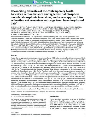
NORTH AMERICAN CARBON BALANCE 5Table 1 (continued)(c) Characteristics (temporal coverage, spatial coverage, variables included, literature reference) of terrestrial biosphere modelestimates used in this studyData type/NameTemporalcoverageSpatial coverageVariables includedin NEELand use (LU)& disturbanceMC12000–2006Continental US (n 49)(Ra Rh)–GPP FirePrescribed LU,prognosticharvest & fireBEPSORCHIDEE2000–20042001–2005North America (n 97)North America (n 97)(Ra Rh)–GPP(Ra Rh)–GPP FireTEM62000–2006North of 45oN (n 14)VEGAS22000–2005North America (n 97)(Ra Rh)–GPP Fire Prod(Ra Rh)–GPP FirePrescribed LU,prognosticharvest & firePrescribed LU,harvest, firePrognostic fireReferenceBachelet et al. (2003)Ju et al. (2006)Krinner et al. (2005)Hayes et al. (2011)Zeng et al. (2005)*includes Alaska.†includes the District of Columbia.‡NEE (and GPP) are empirically derived from MODIS variables.Fig. 1 Conceptual diagram of the continental-scale carbon budget, including the land-atmosphere exchange of CO2 (NEE), based ondata available from the inventory-based approaches that estimate carbon stock changes, fluxes and transfers among forest, crop, andother lands.of HR that was emitted during the processing of harvestedwood into products (HE). This processing, or ‘primary consumption’, was assumed to occur largely at the mill, and sowe allocated this source term within the Forest Lands sector ofthe reporting zone in which the wood was harvested. Theremainder (i.e., HR – HE) was assumed to be transported offsite and added to the national-level forest product pool thatresides in the Other Lands sector (described below).The data set on forest carbon accounting in Canada’s Managed Forest Area used here employed the ‘stock-plus-flow’approach, which starts with data from a compiled set ofinventories and then models the components of change. Fluxdata were produced using the Carbon Budget Model of theCanadian Forest Sector (CBM-CFS3), which uses stand-levelgrowth data to estimate annual carbon uptake along withdetailed annual natural disturbance (e.g., fire, insects) and harvest data to track carbon transfers through the system (Kurzet al., 2009; Stinson et al., 2011). Natural disturbance and harvest removals data were from various provincial-level reporting sources in Canada (Stinson et al., 2011). The stock changeterms (DLive DDOM) as shown in Eqn (2) also includednon-CO2/non-vertical exchanges and these fluxes were separated out of the NEEF calculation. These more detailed component fluxes were estimated by CBM-CFS3, and so NEEF forCanada was calculated from the available indicator variablesas:Published 2011This article is a US Government work and is in the public domain in the USA, Global Change Biology, doi: 10.1111/j.1365-2486.2011.02627.x
6 D. J. HAYES et al.NEEF ¼ DLive þ DDOM ðFireC FireCO2 Þ þ HR þ HE ð3Þwhere the carbon remaining in harvested products after primary consumption (i.e., HR – HE) and the non-CO2 componentof fire emissions (i.e., FireC – FireCO2) were excluded fromthe vertical flux component of the overall stock change. ForCanada, we used 30% as the proportion of HR emitted in primary consumption, based on an analysis of 2010 FAO statistics (FAOStat; http://faostat.fao.org/) and Canadian harvestdata for the period 2000–2006. Therefore: HE is equal to0.3 9 HR for each reporting zone.The forest inventory data sets for the US were based on theforest surveys of the U.S. Department of Agriculture (USDA)Forest Service’s Forest Inventory and Analysis (FIA) program(Bechtold & Patterson, 2005). These estimates were coupledwith carbon expansion factors (Bechtold & Patterson, 2005;Smith et al., 2006; Heath et al., 2011) and estimates of carbonstock changes were derived from the Carbon Calculation Tool(CCT; Smith et al., 2010), which is used to produce the GHGinventory for US forest lands in the UNFCCC reports (EPA,2011). Harvest removals (HR) were from published US ForestService data sets (Smith et al., 2009). Estimates of the proportion of HR emitted in primary consumption (HE) were provided by Smith et al. (2006), who showed that the proportionlost within the first year following harvest (which we assumedoccurs primarily at the mill) ranges from 20% to 40% acrossspecies group and region in the US. As such, we used 30% asa representative emissions (from primary consumption) fraction, which is the same as that used for the Canada data set.State-level data on fire emissions from US forests were notavailable for the time period of this study; however, in termsof our NEE calculation, fire emissions were implicit in the totalstock change (i.e. fire emissions would have accumulated asbiomass had there been no fire) and considered a source ofcarbon to the atmosphere. The US forest data represents netstock change, meaning that fluxes stemming from land usechange (LUC; i.e. forest land area converted to other land use,and other land converted to forest land) were also implicit (i.e.integrated in) in the stock change data. The correspondingchange in carbon stocks directly attributed to fire and LUCcannot be explicitly separated from the total stock change.Therefore, NEEF for the US Forest Lands sector used exactlythat as shown in Eqn (2), without the modification for nonCO2 fire emissions as used in Canada.As with the Canada forest data set, the Mexico inventorydata can be described as being based on the ‘stock-plus-flow’approach. For Mexican forests, the data set was based on acarbon accounting methodology in which mean carbon stockdensity by forest type was distributed according the arealextent of each type at an initial point in time, and stock changewas estimated according to the biomass increment (growth)and harvest amount in managed forests, and area of forestconversion over a subsequent period of time. Using this methodology, the study by deJong et al. (2010) calculated for the1993–2002 time period: (1) biomass losses resulting from theconversion of forests to other land use (DLiveLUC); (2) theassociated change in soil carbon stocks resulting from LUC(DSoilLUC); (3) carbon uptake due to the regrowth of forests onabandoned agricultural or other lands (DLiveABND); and (4)the net carbon balance between uptake (growth) andemissions (harvest) in managed forests (DLiveMNGD). Fireemissions were included with respect to burning in forestconversion, but the reporting methodology does not take intoaccount fire emissions or other natural carbon fluxes (growth,mortality) from unmanaged land. NEEF was calculated bysumming the four average annual stock change componentsfrom the study by deJong et al. (2010):NEEF ¼ DLiveLUC þ DSoilLUC þ DLiveABND þ DLiveMNGD :ð4ÞFor this study, we distributed the magnitude of each component flux proportionately by an estimate of the relative areaof each LU/LC class contained in each state, as described inthe Supporting Information. Without more detailed data, weassumed that commercial harvest and fuelwood harvestoccurred proportional to the relative area of each forest type.Crop lands sector inventoriesTo estimate NEE for croplands for this study, we collected estimates of crop productivity (NPP), harvest (HR) and changes insoil carbon stocks (DSoil) over the 2000–2006 time period forCanada (Environment Canada, 2011) and the US (West et al.,2011). The detail regarding the source and methodologies usedin the crop inventories are provided in the Supporting Information as well as by those references cited. NEEC was calculated for each reporting zone in Canada and the US as:NEEC ¼ DSoil þ HR ;ð5Þwhere all crop harvest removals (i.e., HR) were considered aCrop Lands sector sink in the reporting zone where they wereharvested; unlike the treatment of harvested wood products,we assumed no primary consumption emissions within theCrop Lands sector. We considered DLive in croplands to beequal to zero on an annual basis since the assumption of thedata was that NPP is equal to the crop harvest plus residue.We then assumed that, within the same year, the residue carbon was returned to the atmosphere (via combustion ordecomposition) or incorporated into the soil C pool.Data specific to crop productivity and harvest in Mexicowere not available for this study, and croplands were notmapped separate from other agricultural lands and forestplantations in the study by deJong et al. (2010). As such, wewere not able to report estimates of sources and sinks for theMexican cropland sector separately in this study, but ratherincluded the contribution of soil carbon stock changes fromagricultural establishment and abandonment in the OtherLands sector for Mexico.Other lands sector inventoriesThe Other Lands sector was used in this study to include twoadditional fluxes: (1) net surface carbon fluxes from lands notincluded in Forest Land or Crop Land sectors (i.e. grasslands,settlements and other lands) and (2) CO2 emissions from thePublished 2011This article is a US Government work and is in the public domain in the USA, Global Change Biology, doi: 10.1111/j.1365-2486.2011.02627.x
NORTH AMERICAN CARBON BALANCE 7combustion, decay, and respiration of carbon in harvested forest and crop products. NEEO was calculated for Canada andthe US by combining various component fluxes according tothe following equation:NEEO ¼ NEEG þ NEES þ EH þ EL þ EF ;ð6Þwhich considered the net carbon balance of grassland areas(NEEG), the net carbon balance of human settlement areas(NEES), CO2 emissions from human respiration (EH), CO2emissions from livestock respiration (EL) and CO2 emissionsfrom the decay of harvested forest products (EF). For NEEGand NEES we used general, area-weighted estimates of ‘Grassland’ and per-capita estimates of ‘Settlements/Other’ sinkcategories reported in the EPA GHG inventory for years 2000–2006 (EPA, 2011). We then extrapolated area-weighted NEEGand per-capita NEES according to the area or human population represented by each category in each reporting zone. Thearea of Other Lands in each reporting zone of Canada and theUS is calculated as the remainder of the total area of each zoneafter subtracting the Forest Land and Crop Land areas fromthe inventory data sets. The estimates of the product emissionterms (EH EL EF) are described in the next section and inthe Supporting Information.The data set containing state-level estimates of carbon fluxfrom the Other Lands sector in Mexico was developed usingthe same Eqn (4) as
be a small net source ( 18 TgC yr 1) due to land use change between 1993 and 2002. We compare these inventory-based estimates with results from a suite of terrestrial biosphere and atmospheric inversion models, where the mean continental-scale NEE estimate for each ensemble is 511 TgC yr 1 and 931 TgC yr 1, respectively. In the modeling