Transcription
UNIVERSITY OF MISKOLCFaculty of EconomicsInstitute of Business Information and MethodsDepartment of Business Statistics and Economic ForecastingPETRA PETROVICSSPSS TUTORIAL & EXERCISE BOOKFOR BUSINESS STATISTICSMISKOLC2012
TABLE OF CONTENTI. SPSS Tutorial . 61.Introduction to SPSS . 62.Transform / Select Data. 83.Graphs . 124.Central Tendencies, Measures of Distribution, Measures of Asymmetry . 205.Estimation and Hypothesis Testing . 236.Statistical Dependence . 307.Correlation and Linear Regression . 368.Multiple Correlation and Linear Regression . 429.Curvilinear Regression . 4510. Time Series Analyzes . 48II. Exercises for SPSS. 60
LIST OF FIGURESFigure 1 – Opening an SPSS Data File .6Figure 2 – Variable Type Dialog Box .7Figure 3 – Value Labels Dialog Box .7Figure 4 – Missing Values Dialog Box .8Figure 5 – Compute Variable Dialog Box .9Figure 6 – Frequencies Dialog Box.10Figure 7 – Select Cases Dialog Box .11Figure 8 – Selected Subset of Cases.11Figure 9 – Bar Charts Dialog Box.12Figure 10 – Bar Charts Dialog Box .12Figure 11 – Chart Editor .13Figure 12 – Bar Chart .13Figure 13 – Chart Editor Properties Dialog Box.14Figure 14 – Pie Chart .14Figure 15 – Stacked Bar Chart Dialog Box .15Figure 16 – Stacked Bar Chart .15Figure 17 – Scatter / Dot Dialog Box .16Figure 18 – Simple Scatter Plot Dialog Box.16Figure 19 – Simple Scatter Plot .17Figure 20 – Box Plot.17Figure 21 – Box Plot Dialog Box .18Figure 22 – Box Plot Chart Editor .18Figure 23 – Clustered Box Plot Chart Editor .19Figure 24 – Clustered Box Plot .20Figure 25 – Descriptives Dialog Box .21Figure 26 – Clustered Box Plot .21Figure 27 – Frequencies Statistics Dialog Box .22Figure 28 – One-Sample T Test Dialog Box for Estimation .23Figure 29 – One-Sample T Test Dialog Box for Hypothesis Testing .24Figure 30 – Independent Samples T Test Dialog Box .25Figure 31 – One-Sample Kolmogorov–Smirnov Test Dialog Box .26Figure 32 – Histogram Dialog Box .28Figure 33 – Histogram .28Figure 34 – Two-Independent-Samples Tests Dialog Box.29Figure 35 – Crosstabs Dialog Box .30Figure 36 – Cell Display Dialog Box .31Figure 37 – Crosstabs Statistics Dialog Box .32Figure 38 – Chi-square Distribution.33Figure 39 – Means Dialog Box .34Figure 40 – Means Options Dialog Box .34Figure 41 – Bivariate Correlations Dialog Box .36Figure 42 – Linear Regression Dialog Box .37Figure 43 – Linear Regression: Statistics Dialog Box .38Figure 44 – Linear Regression Dialog Box: Statistics for Estimating the Coefficients .40Figure 45 – Linear Regression: Save for Prediction Intervals .41Figure 46 – Multiple Linear Regression .43Figure 47 – Curve Estimation Dialog Box .46
Figure 48 – Curve Fit .47Figure 49 – Sequence Charts Dialog Box.49Figure 50 – Sequence Chart .50Figure 51 – Curve Estimation for Linear Trend Model .50Figure 52 – Curve Estimation: Save Dialog Box .51Figure 53 – Predicted Number of Birth .52Figure 54 – Define Dates Dialog Box .53Figure 55 – Sequence Chart Dialog Box .53Figure 56 – Time Axis Reference Line Dialog Box .54Figure 57 – Time Axis Reference Line Dialog Box .54Figure 58 – Seasonal Decomposition Dialog Box .55Figure 59 – Seasonal Decomposition Dialog Box .56Figure 60 – Error Component .56Figure 61 – SAF 1: Seasonal Component.57Figure 62 – SAS 1: Component without Seasonality .57Figure 63 – STC 1: Smoothed Trend-cycle Component .58Figure 64 – Forecasted Values .59Figure 65 – Predicted Railway Transport .59
INTRODUCTIONThis exercise book was written for the students of the University of Miskolc within theframework of Business Statistics and Quantitative Statistical Methods. Some parts of theexercises are translated from the Hungarian book of Domán – Szilágyi – Varga: Statisztikaielemzések alapjai II, which are supplemented by SPSS exercises on the basis of SPSS 16.0and 19.0 Tutorial. This book is a tutorial, which includes theoretical background just tounderstand the examples included.ACKNOWLEDGEMENTSThe described work was carried out as part of the TÁMOP-4.2.1.B-10/2/KONV-2010-0001project in the framework of the New Hungarian Development Plan. The realization of thisproject is supported by the European Union, co-financed by the European Social Fund.
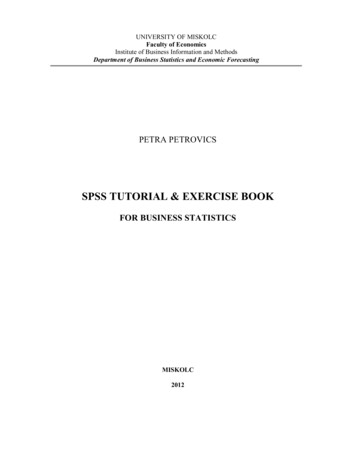
6I. SPSS TUTORIAL1. INTRODUCTION TO SPSS1Open the Csernely data.sav file!Figure 1 – Opening an SPSS Data FileThe Data Editor provides 2 views of data: the Data View and Variable View. Information canbe edited or deleted in both views.Data View: this view displays the actual data values or value labels.Variable View: Name: it is a unique name of each variable (the names should be different). The namescannot contain space or other illegal characters and the first character must be aletter. Type: it specifies the type of data for each variable. The original setting is the mostfrequently used type, the numeric type, which refers to variable, whose valuesare numbers. However, we can change to Comma, Dot, Scientific Notation,Date, Dollar, Custom Currency or String Variables.1According to SPSS 16.0 Tutorial
7SPSS TutorialFigure 2 – Variable Type Dialog Box Width: the field width. Decimals: number of decimals in case of Numeric type. Label: descriptive name of a variable (up to 256 characters). It can contain space orother characters, which we could not use in Names. Values: we can assign descriptive value labels for each value of a variable, thus thenumeric codes represent non-numeric categories.Figure 3 – Value Labels Dialog Box Missing: if we do not have data, because e.g. a respondent refused to answer. Usermissing values are flagged for special treatment and are excluded from mostcalculations.
8SPSS TutorialFigure 4 – Missing Values Dialog Box Column: number of characters for the column width. Align: alignment controls the display of data. It can be right, left or center. Measures: it is the scales of measurement, which can be nominal, ordinal, interval orratio scale. In the SPSS you will find the nominal, ordinal and ratiomeasures. Nominal scale: Numbers are labels or groups or classes. Simple codes assignedto objects as labels. We use nominal scale for qualitative data, e.g. professionalclassification, geographic classification. E.g. blonde: 1, brown: 2, red: 3, black:4. A person with red hair does not possess more ‘hairiness’ than a person withblonde hair. Ordinal scale: Data elements may be ordered according to their relative size orquality, the numbers assigned to objects or events represent the rank order (1st,2nd, 3rd etc.) E.g. top lists of companies. Interval scale: There is a meaning of distances between any two observations.The "zero point" is arbitrary. Negative values can be used. Ratios betweennumbers on the scale are not meaningful, so operations such as multiplicationand division cannot be carried out directly. E.g. temperature with the Celsiusscale. Ratio scale (Scale): This is the strongest scale of measurement. Distancesbetween observations and also the ratios of distances have a meaning. Itcontains a meaningful zero. E.g. mass, length.2. TRANSFORM / SELECT DATAExample 1 How old are the respondents? Create a new variable as age!We can create new variables by transforming another one. We have data about the date ofbirth of employees. If we subtract the year of birth from the current year, we will get their age.In order to determine the age, choose Transform / Compute Variable from the menus.
9SPSS TutorialFigure 5 – Compute Variable Dialog BoxType the name of target variable, say age. To build an expression, type components directly inthe Expression field. If the date of birth is given as Date (mm/dd/yyyy), we need just the yearpart of this. Thus we should extract date.When we are ready with the expression, press OK, then the new variable will be ready.Example 2 What is the proportion of single people?From the menus choose: Analyze / Descriptive Statistics / Frequencies Select the variable,which relative frequency should be calculated (Marital status), and then press OK.
10SPSS TutorialFigure 6 – Frequencies Dialog BoxFind the results in the Output View.Marital r (but not 474.0100.0Therefore, 5.4% of people are single in Csernely. (5.5% of respondents are single.)Example 3 What is the proportion of men within pensioners?Now, the statistical population is not the respondents, but just pensioners. First we shouldselect the subset of cases (pensioner) with Data / Select cases
11SPSS TutorialFigure 7 – Select Cases Dialog BoxWe use a conditional expression to select men: Gender 1 (because 1 is the code of men).Figure 8 – Selected Subset of CasesThen choose Analyze / Descriptive Statistics / Frequencies The relative frequencies ofgender are the question, so Gender should be added to Variables. The following are the resultsfound in the Output view:GenderValidFrequencyPercentValid PercentCumulative 23100.0100.050.4% of pensioners are men.
12SPSS Tutorial3. GRAPHSExample 1Create a bar chart about the proportion of respondents grouped by gender! Embellish thegraph! Attach the value of proportions to the chart!For creating a bar chart, choose Graphs / Legacy Dialogs / Bar Charts / Simple from menus.Figure 9 – Bar Charts Dialog BoxThen select a variable for the category axis (gender). The question was about the proportionof respondents, therefore bars should represent % of cases.Figure 10 – Bar Charts Dialog Box
13SPSS TutorialGraph is stored in the Output window. To edit a Legacy Dialogs graph, double click on thegraph, a Chart Editor window appears. Alternatively, you can also right-click on the chart andselect Edit Content and then select ‘In separate window’.2Optionally, you can change the proportions of the chart: e.g. colour, depth and angle (3D),width of bars, etc. For attaching the proportion values to the chart, select Data Label Mode, ason the Figure below.Figure 11 – Chart EditorFigure 12 – Bar Chart2SPSS Online Training Workshop, Central Michigan University (accessed: 05-01-2011)
14SPSS TutorialExample 2 Transform the bar chart into a pie chart!In order to transform a chart, click the previously edited bar chart in the Chart Editor andselect the Properties from the menus: Edit / Properties / Variables / Element Type Figure 13 – Chart Editor Properties Dialog BoxFigure 14 – Pie ChartExample 3Create a column diagram about the proportion of respondents grouped by education levelstacked by gender! Embellish the graph!
15SPSS TutorialThe only difference between Example 1 and 3 is that now we should create stacked bar chart.Bar chart can be obtained by clicking on Graphs menu and selecting Legacy Dialogs / BarCharts and then selecting the stacked type of bar chart (as on Figure 13). Then definecategory axis (Education level) and stacks (Gender).Figure 15 – Stacked Bar Chart Dialog BoxFigure 16 – Stacked Bar Chart
16SPSS TutorialExample 4Create a scatter plot of average income and total expenditure of households if you set markersby the type of heating (heating bin)! Embellish the graph!Scatter plot can be obtained by clicking on Graphs / Legacy Dialogs / Scatter/Dot , and thenthe following box will appear. Simple scatter plot should be chosen.Figure 17 – Scatter / Dot Dialog BoxFigure 18 – Simple Scatter Plot Dialog BoxFirst we should define the axes (x: average income; y: total expenditure), then set markers bythe type of heating (heating bin). Optionally, we can label cases by a variable. If we have thenames of respondents, that would be the label. Using the Chart Editor, we also can embellishthe chart (change the colour or the type of markers).
17SPSS TutorialFigure 19 – Simple Scatter PlotExample 5 Define a horizontal box plot of total expenditure! Embellish the graph!First of all, we should define, what a box plot means. The box plot is a set of summarymeasures of distributions, like median, lower quartile, upper quartile, the smallest and thelargest observations, moreover, the asymmetry can be seen as well.Figure 20 – Box PlotSource: Aczel, 1996
18SPSS TutorialTurning back to the exercise, we should create a box plot: Graphs / Legacy Dialogs / Boxplot.Choose simple chart to create a plot of one variable, and clustered for a comparison ofvariable types. Now we need a simple box plot of current salary, where data are summaries ofseparate variables.Figure 21 – Box Plot Dialog BoxFor a horizontal box plot we need to transpose the chart: Chart Editor / Options / TransposeChart.Figure 22 – Box Plot Chart Editor
19SPSS TutorialExample 6Define box plot of total expenditure of households categorized by the type of heating(heating bin) clustered by household clusters! Embellish the graph!For a categorized chart, choose the clustered box plot, where data in chart are summaries forgroups of cases. The selected variable is the total expenditure and the type of heating(heating bin) is on the category axis. The clusters are defined by household clusters.Figure 23 – Clustered Box Plot Chart EditorThe graph is edited by double clicking on the graph and double clicking on the part of graphwhich wanted to be edited. Then a Properties dialog box will appear to make changes. Aftermaking the changes, click on Apply to effect the changes and then close the dialog box.
20SPSS TutorialFigure 24 – Clustered Box Plot4. CENTRAL TENDENCIES, MEASURESASYMMETRYOFDISTRIBUTION, MEASURESOFExampleDefine the central tendencies, measures of distribution, measures of asymmetry and quartilesfor total expenditure (HUF/month) of households!These are measures of descriptive statistics, which are obtained by clicking on Analyze menuand selecting Descriptive Statistics then Descriptive.Select the variable, which should be analyzed. If we would like, we can standardize variablesas well, as it is shown on the figure below.
21SPSS TutorialFigure 25 – Descriptives Dialog BoxClick on Options for optimal statistics.Figure 26 – Clustered Box PlotUsing this option we can define mean, standard deviation and the measure of asymmetry.
22SPSS TutorialAlternatively, we reach descriptive statistics from Analyze / Descriptive Statistics /Frequencies menu. After clicking on Statistics, the following box will appear:Figure 27 – Frequencies Statistics Dialog BoxThe results are stored in the Output window.StatisticsTotal expenditure 0.00Mode58500.00aStd. 0075126700.00a. Multiple modes exist. The smallest value is shownThe following are interpretations of figures:
23SPSS Tutorial 222 households were examined in Csernely. (Number of cases) The average monthly expenditure is 99 692.72 HUF. Half of the households spend more than 85 500 HUF, the other half of them spendless. (85 500 HUF is the value above and below which half of the cases fall.) The most frequently occurring monthly expenditure is 58 500 HUF. Multiple modeexist and 58 500 HUF is the smallest value. The average dispersion around the mean is 57045.35 HUF. Long right tail asymmetry. (A distribution with a significant positive skewness has along right tail.) Positive kurtosis indicates that the observations cluster more and have longer tails thanthose in the normal distribution. The lowest total expenditure of households is 5 000 HUF. The highest total expenditure of households is 337 000 HUF. 25% of households have lower monthly expenditure than 59 875 HUF and 75% havehigher. 75% of households have lower monthly expenditure than 126 700 HUF and 25% havehigher.5. ESTIMATION AND HYPOTHESIS TESTINGExample 1 Define a 95% confidence interval for the total expenditure!For defining a confidence interval, t-test is available in the SPSS by clicking on Analyze /Compare Means / One Sample T Test Figure 28 – One-Sample T Test Dialog Box for EstimationIn case of estimation, the test value should be zero.Optionally, click on Options to control the confidence level. (The original setting is 95%).After clicking on OK, the results will be appeared in the Output window.
24SPSS TutorialTest Value 0t26.039df221Sig. (2tailed)MeanDifference0.000 99692.7162295% Confidence Interval of theDifferenceLower92147.4136Upper107238.0189The average total expenditure of households is between 92 147.4136 and 107 238.0189 HUFat 95% confidence level.Example 2Test the hypothesis that the total expenditure of households equals 100 000. (α 5%)From the menu choose Analyze / Compare Means / One Sample T Test Enter the test value which each mean sample is compared. This is 100 000, as you can seebelow.Figure 29 – One-Sample T Test Dialog Box for Hypothesis TestingIf the significance level is 5%, the confidence level will be 95%, which can be edited underthe Options menu.The results are the following:t-.080df221Test Value 10000095% Confidence Interval of r-7852.58647238.0189.936 -307.28378
25SPSS TutorialIf the p-value is less than 0.05, we reject the null. The p-value is 0.936, so we are basicallydeclaring the null hypothesis to be true.Example 3Test the hypothesis that the average expenditure on heating of households heating with gasand households heating with solid fuels are equal! (α 5%)For comparing two independent means use independent t-test by clicking on Analyze /Compare Means / Independent Samples T Test Figure 30 – Independent Samples T Test Dialog BoxSelect the type of heating (heating bin) as a grouping variable, where the groups are gas andsolid fuels (coded as 1 and 2). Cases with any other values are excluded from the analysis.By clicking on Options, the confidence level can be changed.If the population standard deviations are unknown, we have an assumption for equality ofvariances. Levene’s test controls the equality of variances.Levene's Test forEquality of VariancesEqual variancesassumedEqual variancesnot assumedt-test for Equality of MeansFSig.tdfSig.(2-tailed)MeanStd. ErrorDifference .716189.9900.088-5617.63273.48We should analyze the first row, because equal variances assumed, because ngas 71 andnsolid fuel 121 (small sample size). When the F-value is large and the significance level ofLevene’s Test is small (smaller than say 0.1) the hypothesis of equal variances can be
26SPSS Tutorialrejected. The assumption is not significantly satisfied thus we cannot analyze the results of ttest. Anyway, we are basically declaring the alternative hypothesis to be true. Typically aconditional probability (critical significance level) of less than 0.1 or 0.05 is consideredsignificant, thus the average expenditure on heating of households heating with gas or solidfuels are not equal.Example 4 Nonparametric Tests – Hypothesis Testing for DistributionProblem: Test the normality of average expenditure on heating! α 5%Many parametric tests require normally distributed variables, thus we should test thehypotheses, whether the variable follows normal distribution or not.H0: Normal distributionH1: Not normal distributionNonparametric hypothesis testing was applied to test for a normal distribution, that is why wewill find this by clicking on Analyze / Nonparametric tests / 1-Sample K-S Test in the SPSS.One-Sample Kolmogorov – Smirnov Test procedure compares the observed cumulativedistribution function for a variable with a specified theoretical distribution, which can benormal as well.Figure 31 – One-Sample Kolmogorov–Smirnov Test Dialog BoxThe test variable is now the average expenditure on heating and the test distribution is normal.If we want, we can generate descriptive statistics (usually including mean, standard deviation,sample size, minimum and maximum values, etc) by clicking on Options. It is good to know
SPSS Tutorial27them, because this procedure estimates the parameters from the sample, where the samplemean and standard deviation are the parameters for a normal distribution.The following are the result in the Output View:One-Sample Kolmogorov-Smirnov TestAverage expenditure on heating(HUF/month)N193Normal Parametersa,b Mean31727.10Std. Deviation25014.693Most -.122Kolmogorov-Smirnov Z2.290Asymp. Sig. (2-tailed).000a. Test distribution is Normal.b. Calculated from data.The p-value (asymp. sig.) tells you the probability of getting the results you got if the nullwere actually true. Thus the probability you would be in error if you rejected the nullhypothesis is 0%. In other words, if the p-value is less than 0.05, you reject the normalityassumption. So the average monthly expenditure on heating does not follow normaldistribution.Alternatively, there is another way of testing the normal distribution: using a histogram. Thegraph of the normal distribution depends on two factors - the mean and the standard deviation.The mean of the distribution determines the location of the center of the graph, and thestandard deviation determines the height and width of the graph. When the standard deviationis large, the curve is short and wide; when the standard deviation is small, the curve is tall andnarrow. All normal distributions look like a symmetric, bell-shaped curve.3From the menus choose Graphs / Legacy Dialogs / Histogram, and then the following boxwill appear:3Statistics Tutorial: http://stattrek.com (accessed: 05-01-2011)
28SPSS TutorialFigure 32 – Histogram Dialog BoxFigure 33 – HistogramTherefore, the average monthly expenditure on heating is not normally distributed, because atruly normal curve is shaped like a bell that peaks in the middle and is perfectly symmetrical.
29SPSS TutorialExample 5Test the hypothesis, that average expenditure on heating of households heating with gas andhouseholds heating with solid fuels are equal, if we know that the average expenditure onheating does not follow normal distribution.H0: The average expenditure on heating of households heating with gas and householdsheating with solid fuels are equal.H1: The average expenditure on heating of households heating with gas and householdsheating with solid fuels are not equal.In case of a non-normally distributed variable, we should use a nonparametric test forhypothesis testing. From the menus choose Analyze / Nonparametric tests / 2-IndependentSamples and then the following dialog box will appear:Figure 34 – Two-Independent-Samples Tests Dialog BoxSelect the average expenditure on heating for test variable and heating category (heating bin)for grouping variable. Click on Define Groups to split the file into two groups: Group 1:mainly gas (coded 1), Group 2: solid fuel (coded 2).Mann-Whitney U Test is the most popular two-independent-samples test.The following are the results from the Output window:Test StatisticsaAverage expenditure on heating(HUF/month)Mann-Whitney U4020.000Wilcoxon W6576.000Z-.743Asymp. Sig. (2-tailed).458a. Grouping Variable: Gas or solid fuel
30SPSS TutorialThe p-value is less than 0.1, so we reject the null hypothesis. The salary of clericals andmanagers are not equal.6. STATISTICAL DEPENDENCEExample 1 Create crosstabs from the type of heating (heating bin) and household clusters!Cross tabulation is the process of creating a contingency table from the multivariate frequencydistribution of statistical variable. From the menus choose Analyze / Descriptive Statistics /Crosstabs.Figure 35 – Crosstabs Dialog BoxSelect the row and column variable. It is up to you, which one is selected for row or column.By clicking on cells, percentages or residuals can be displayed as well, as it is shown on thefigure below.
31SPSS TutorialFigure 36 – Cell Display Dialog BoxTherefore, each cell of the statistical table can
I. SPSS TUTORIAL 1. INTRODUCTION TO SPSS 1 Open the Csernely_data.sav file! Figure 1 - Opening an SPSS Data File The Data Editor provides 2 views of data: the Data View and Variable View. Information can be edited or deleted in both views. Data View: this view displays the actual data values or value labels. Variable View: