Transcription
Projective Geometry: A Short IntroductionLecture NotesEdmond Boyer
Master MOSIGIntroduction to Projective GeometryContents1 Introduction1.1 Objective . . . . . . . . . . . . . . . . . . . . . . . . . . . . . . .1.2 Historical Background . . . . . . . . . . . . . . . . . . . . . . . .1.3 Bibliography . . . . . . . . . . . . . . . . . . . . . . . . . . . . .22342 Projective Spaces2.1 Definitions . . . . . . . . . . . . . . . . . . . . . . . . . . . . . . .2.2 Properties . . . . . . . . . . . . . . . . . . . . . . . . . . . . . . .2.3 The hyperplane at infinity . . . . . . . . . . . . . . . . . . . . . .558123 The3.13.23.3projective line13Introduction . . . . . . . . . . . . . . . . . . . . . . . . . . . . . . 13Projective transformation of P 1 . . . . . . . . . . . . . . . . . . . 14The cross-ratio . . . . . . . . . . . . . . . . . . . . . . . . . . . . 144 The4.14.24.34.44.54.64.74.8projective planePoints and lines . . . . . .Line at infinity . . . . . .Homographies . . . . . . .Conics . . . . . . . . . . .Affine transformations . .Euclidean transformationsParticular transformationsTransformation hierarchyGrenoble Universities.1717181920222224251
Master MOSIGIntroduction to Projective GeometryChapter 1Introduction1.1ObjectiveThe objective of this course is to give basic notions and intuitions on projectivegeometry. The interest of projective geometry arises in several visual computing domains, in particular computer vision modelling and computer graphics.It provides a mathematical formalism to describe the geometry of cameras andthe associated transformations, hence enabling the design of computational approaches that manipulates 2D projections of 3D objects. In that respect, afundamental aspect is the fact that objects at infinity can be represented andmanipulated with projective geometry and this in contrast to the Euclideangeometry. This allows perspective deformations to be represented as projectivetransformations.Figure 1.1: Example of perspective deformation or 2D projective transformation.Another argument is that Euclidean geometry is sometimes difficult to use inalgorithms, with particular cases arising from non-generic situations (e.g. twoparallel lines never intersect) that must be identified. In contrast, projectivegeometry generalizes several definitions and properties, e.g. two lines alwaysintersect (see fig. 1.2). It allows also to represent any transformation that preserves coincidence relationships in a matrix form (e.g. perspective projections)that is easier to use, in particular in computer programs.Grenoble Universities2
Master MOSIGIntroduction to Projective GeometryInfinitynon-parallel linesparallel linesFigure 1.2: Line intersections in a projective space1.2Historical BackgroundThe origins of geometry date back to Egypt and Babylon (2000 BC). It wasfirst designed to address problems of everyday life, such as area estimations andconstruction, but abstract notions were missing. around 600 BC: The familiar form of geometry begins in Greece. Firstabstract notions appear, especially the notion of infinite space. 300 BC: Euclide, in the book Elements, introduces an axiomatic approach to geometry. From axioms, grounded on evidences or the experience, one can infer theorems. The Euclidean geometry is based on measures taken on rigid shapes, e.g. lengths and angles, hence the notion ofshape invariance (under rigid motion) and also that (Euclidean) geometricproperties are invariant under rigid motions. 15th century: the Euclidean geometry is not sufficient to model perspective deformations. Painters and architects start manipulating the notionof perspective. An open question then is ”what are the properties sharedby two perspective views of the same scene ?” 17th century: Desargues (architect and engineer) describes conics as perspective deformations of the circle. He considers the point at infinity asthe intersection of parallel lines. 18th century: Descartes, Fermat contrast the synthetic geometry of theGreeks, based on primitives with the analytical geometry, based instead oncoordinates. Desargue’s ideas are taken up by Pascal, among others, whohowever focuses on infinitesimal approaches and Cartesian coordinates.Monge introduces the descriptive geometry and study in particular theconservation of angles and lengths in projections. 19th century : Poncelet (a Napoleon officer) writes, in 1822, a treaty onprojective properties of figures and the invariance by projection. This isthe first treaty on projective geometry: a projective property is a property invariant by projection. Chasles et Möbius study the most generalGrenoble Universities3
Master MOSIGIntroduction to Projective Geometryprojective transformations that transform points into points and lines intolines and preserve the cross ratio (the collineations). In 1872, Felix Kleinproposes the Erlangen program, at the Erlangen university, within whicha geometry is not defined by the objects it represents but by their transformations, hence the study of invariants for a group of transformations.This yields a hierarchy of geometries, defined as groups of transformations,where the Euclidean geometry is part of the affine geometry which is itselfincluded into the projective geometry.Projective GeometryAffine GeometryEuclidean GeometryFigure 1.3: The geometry hierarchy.1.3BibliographyThe books below served as references for these notes. They include computervision books that present comprehensive chapters on projective geometry. J.G. Semple and G.T. Kneebone, Algebraic projective geometry, ClarendonPress, Oxford (1952) R. Hartley and A. Zisserman, Multiple View Geometry, Cambridge University Press (2000) O. Faugeras and Q-T. Luong, The Geometry of Multiple Images, MITPress (2001) D. Forsyth and J. Ponce, Computer Vision: A Modern Approach, PrenticeHall (2003)Grenoble Universities4
Master MOSIGIntroduction to Projective GeometryChapter 2Projective SpacesIn this chapter, formal definitions and properties of projective spaces are given,regardless of the dimension. Specific cases such as the line and the plane arestudied in subsequent chapters.2.1DefinitionsConsider the real vector space Rn 1 of dimension n 1. Let v be a non-zeroelement of Rn 1 then the set Rv of all vectors kv, k R is called a ray (cf.figure 2.1).kvFigure 2.1: The ray Rv is the set of all non-zero vectors kv with direction v.Definition 2.1 (Geometric Definition) The real projective space P n , of dimension n, associated to Rn 1 is the set of rays of Rn 1 . An element of P n is calleda point and a set of linearly independent (respectively dependent) points of P nis defined by a set of linearly independent (respectively dependent) rays.Grenoble Universities5
Master MOSIGIntroduction to Projective GeometryRBRARCBCAFigure 2.2: The projective space associated to R3 is called the projective planeP 2.Definition 2.2 (Algebraic Definition) A point of a real projective space P n isrepresented by a vector of real coordinates X [x0 , ., xn ]t , at least one ofwhich is non-zero. The {xi }s are called the projective or homogeneous coordinates and two vectors X and Y represent the same point when there exists ascalar k R such that:xi kyi i,which we will denote by:X Y.Hence the projective coordinates of a point are defined up to a scale factorand the correspondence between points and coordinate vectors is not one-to-one.Projective coordinates relate to a projective basis:Definition 2.3 (Projective Basis) A projective basis is a set of (n 2) pointsof P n , no (n 1) of which are linearly dependent. For example: 1001 0 1 0 1 . . . . . . . . . . . . . 0011A0A1.AnA Grenoble Universities6
Master MOSIGIntroduction to Projective Geometryis the canonical basis where the {Ai }s are called the basis points and A the unitpoint.The relationship between projective coordinates and a projective basis is asfollows.Projective Coordinates Let {A0 , ., An , A } be a basis of P n with associatedrays Rvi and Rv respectively. Then for any point A of P n with an associatedray Rv , its projective coordinates [x0 , ., xn ]t are such that:v x0 v0 . xn vn ,where the scales of the vectors {vi }s associated to the {Ai }s are given by:v v0 . vn ,which determines the {xi }s up to a scale factor.Note on projective coordinatesTo better understand the above characterization of the projective coordinates, let us consider any (n 1) vectors vi associated to the {Ai }s.By definition they form a basis of Rn 1 and any vector v in this spacecan be uniquely decomposed as:v u0 v0 . un vn , ui R i.Thus v is determined by a single set of coordinates {ui } in the vectorbasis {vi }. However the above unique decomposition with the ui ’s doesnot transfer to the associated points A and {Ai }s of P n since the correspondence between points in P n and vectors in Rn 1 is not one-to-one.For instance replacing in the decomposition u0 by u0 /2 and v0 by 2v0still relates A with the {Ai }s but with a different set of {ui }s. In orderto uniquely determine the decomposition, let us consider the additionalpoint A and let v be one of its associated vector in Rn 1 then:v u 0 v0 . u n vn v 0 . v n .The above scaled vectors v i are well defined as soon as ui 6 0, i (trueby the fact that, by definition, A is linearly independent of any subsetof n points Ai ). Then, any vector v associated to A writes:v x0 v 0 . xn v n ,where the {xi }s can vary only by a global scale factor function of thescales of v and v .Grenoble Universities7
Master MOSIGIntroduction to Projective GeometryDefinition 2.4 (Projective Transformations) A matrix M of dimensions (n 1) (n 1) such that det(M ) 6 0, or equivalently non-singular, defines a lineartransformation from P n to itself that is called a homography, a collineation ora projective transformation.Projective transformations are the most general transformations that preserve incidence relationships, i.e. collinearity and concurrence.2.2PropertiesSome classical and fundamental properties of projective spaces folllow.Theorem 2.1 Consider m points of P n that are linearly independent withm n. The set of points in P n that are linearly dependent on these m pointsform a projective space of dimension m 1. When this dimension is equal to 1,2 and n 1, this space is called line, plane and hyperplane respectively. The setof subspaces of P n with the same dimension is also a projective space.Examples Lines are hyperplanes of P 2 and they form a projective space ofdimension 2.Theorem 2.2 (Duality) The set of hyperplanes of a projective space P n is aprojective space of dimension n. Any definition, property or theorem that appliesto the points of a projective space is also valid for its hyperplanes.2 lines define a point2 points define a lineFigure 2.3: Lines and points are dual in P 2 .Examples Points and lines are dual in the projective plane, 2 points definea line is dual to 2 lines define a point. Another interesting illustration of theduality is the Desargues’ theorem (see figure 2.4) that writes:If 2 triangles are such that the lines joining their corresponding verticesare concurrent then the points of intersections of the corresponding edges areGrenoble Universities8
Master MOSIGIntroduction to Projective Geometrycollinear,and which reciprocal is its dual (replace in the statement lines joining withpoints of intersections of, vertices with edges and concurrent with collinear andvice versa).Figure 2.4: Desargues’ theorem illustrated with parallel lines (hence concurrentlines in the projective sense) joining the corresponding vertices on 2 triangles.Theorem 2.3 (Change of Basis) Let {X0 , ., Xn 1 } be a basis of P n , i.e. no(n 1) of them are linearly dependent. If {A0 , ., An 1 A } is the canonicalbasis then there exists a non-singular matrix M of dimension (n 1) (n 1)such that:M · Ai ki Xi , ki R i,or equivalently:M · Ai Xi i.2 matrices M and M 0 that satisfy this property differ by a non-zero scalar factoronly, which we will denote using the same notation: M M 0 .Grenoble Universities9
Master MOSIGIntroduction to Projective GeometryProofThe matrix M satisfies: M · Ai ki Xi i. Stacking A0 , ., An into amatrix we get, by definition of the canonical basis:[A0 .An ] In 1hence:M · [A0 .An ] M [k0 X0 .kn XN ],which determines M up to the scale factors {ki }. Using this expressionwith An 1 : 1k0 . . . . M · An 1 [k0 X0 .kn XN ] · [X0 .XN ] · . , . 1knand since: M · An 1 kn 1 Xn 1 we get: k0 . . kn 1 Xn 1 ,[X0 .XN ] · . knthat gives the {ki }s up to a single scale factor. Note also that the {ki }sare necessarily non-zero otherwise (n 1) vectors Xi are linearly dependent by the above expression.Thus any basis of P n is related to the canonical basis by a homography. Aconsequence of theorem 2.3 is that:Corollary 2.4 Let {X0 , ., Xn 1 } and {Y0 , ., Yn 1 } be 2 basis of P n , thenthere exists a non-singular matrix M of dimension (n 1) (n 1) such that:M · Xi Yi i,where M is determined up to a scale factor.Grenoble Universities10
Master MOSIGIntroduction to Projective GeometryProofBy theorem 2.3:L · Ai ki Xi , i,Q · Ai li Yi , i.Thus:QL 1 · Xi liYi , i,kiand the matrix M QL 1 is therefore such that:M · Xi Yi , i,Now if there is a matrix M 0 such that: M 0 · Xi Yi , i, then replacingXi we get:M 0 L · Ai Yi , i,and by theorem 2.3: M 0 L M L, hence M 0 M .BAA'CB'C'Figure 2.5: Change of basis in P 2 or projective transformation between A, B, Cand A0 , B 0 , C 0 .Figure 2.5 illustrates the change of basis in P 2 . A, B, C and A0 , B 0 , C 0 are 2different representations of the same rays and are thus related by a homography(projective transformation). Note that this figure illustrates also the relationshipbetween coplanar points and their images by a perspective projection.Grenoble Universities11
Master MOSIG2.3Introduction to Projective GeometryThe hyperplane at infinity[X 0,X 1,0]k 0[X0 /k,X1 /k,1]Figure 2.6: In P 2 any line L is the hyperplane at infinity for the affine spaceP 2 \L. In this affine space, all lines that share the same direction are concurrenton the line at infinity.The projective space P n can also be seen as the completion of a hyperplaneH of P n and the set complement An P n \ H. An is then the affine spaceof dimension n (associated to the vector space Rn ) and H is its hyperplane atinfinity also called ideal hyperplane. This terminology is used since H is thelocus of points in P n where parallel lines of An intersect.As an example, assume that [x0 , ., xn ]t are the homogeneous coordinatesof points in P n and consider the affine space An of points with inhomogeneous coordinates (not defined up to scale factor) [x0 , ., xn 1 ]t . Then the locus of points in P n that are not reachable within An is the hyperplane withequation xn 0. To understand this, observe that there is a one-to-onemapping between points in An and points in P n with homogeneous coordinates [x0 , ., xn 1 , 1]t . Going along the direction [x0 , ., xn 1 ]t in An by changing the value of k in [x0 /k, ., xn 1 /k, 1]t we see that there is a point at thelimit k 0, that is at infinity and not in An , with homogeneous coordinates[x0 /k, ., xn 1 /k, 1]t [x0 , ., xn 1 , k]t k 0 [x0 , ., xn 1 , 0]t (see Figure 2.6).This point belongs to the hyperplane at infinity (or the ideal hyperplane) associated with An .Any hyperplane H of P n is thus the plane at infinity of the affine space P n \H. Reciprocally, adding to any n-dimensional affine space An the hyperplaneof its points at infinity converts it into a projective space of dimension n. Thisis called the projective completion of An .Grenoble Universities12
Master MOSIGIntroduction to Projective GeometryChapter 3The projective lineThe space P 1 is called the projective line. It is the completion of the affineline with a particular projective point, the point at infinity, as will be furtherdetailed in this chapter. The projective line is useful to introduce projectivenotions, such as the cross-ratio, in a simple and intuitive way.3.1IntroductionThe canonical basis of P 1 is: 10A0 , A1 ,01 A A1 A2 11 .A point of P 1 is represented by a vector of 2 homogeneous coordinates X [x0 , x1 ] 6 [0, 0]. Hence: X x0 A0 x1 A1 .Now consider the subspace of P 1 such that x1 6 0. This is equivalent toexclude the point A0 and it defines the affine line A1 . Point on A1 can bedescribed by a single parameter k such that:X kA0 A1 ,where k x0 /x1 is the affine coordinate. OBC Figure 3.1: On the affine line, the coordinate k of C in the coordinate frame[O, B] is k OC/OB.A0 is the point at infinity, or ideal point, for the affine space P 1 \ A0 .Grenoble Universities13
Master MOSIG3.2Introduction to Projective GeometryProjective transformation of P 1A projective transformation of P 1 is represented by a 2 2 non singular matrixH defined up to a scale factor: h1 h2H .h3 h4 The above matrix has 3 degrees of freedom since it is defined up to a scalefactor. From corollary 2.3 of section 2.2, it follows that 3 point correspondences,or equivalently 2 basis of P 1 , are required to estimate H.H Figure 3.2: A homography in P 1 is defined by 3 point correspondences, concerning possibly the infinite point.The restriction of the projective transformation H to the affine space A1 isa transformation M that does not affect the point at infinity, i.e. M · A0 A0 .Hence M is of the form: m1 m2M ,01where m1 is a scale factor and m2 a translation parameter. 2 point correspondences are sufficient to estimate M .3.3The cross-ratioThe cross-ratio, also called double ratio (”bi-rapport” in French), is the fundamental invariant of P 1 , that is to say a quantity that is preserved by projectivetransformation. It is the projective equivalent to the Euclidean distance withrigid transformations. Let A, B, C, D be 4 points on the projective line thentheir cross-ratio writes:{A, B; C, D} AC BD , BC AD xAxBBA B00 (xAA0 x1 ) (x1 x0 ).x1 xB1Some remarks are in order:where AB detGrenoble Universities14
Master MOSIGIntroduction to Projective GeometryABD'C'B'A'CDFigure 3.3: A, B, C, D and A0 , B 0 , C 0 , D0 are related by a projective transformation, hence their cross-ratios are equal.1. The cross-ratio is independent of the basis chosen for P 1 .2. On the affine line, A [ka , 1], B [kb , 1], etc. and the cross-ratio becomes:(kA kC )(kB kD ),{A, B; C, D} (kB kC )(kA kD )hence in the Euclidean space:{A, B; C, D} dAC dBD,dBC dADwith d{} being the Euclidean distance between 2 points.3.{ , B; C, D} (kB kD ),(kB kC ){A, ; C, D} (kA kC ),(kA kD ).4. By permuting the points A, B, C, D, 24 quadruplets can be formed. Thesequadruplets define only 6 different values of the cross-ratio: ρ, ρ1 , 1 ρ1ρ, 1 ρ, ρ 1, ρ 1ρ .5. Let A0 , A1 , A2 be a basis of P 1 and [x0 , x1 ] the coordinates of P in thisbasis, then:x0{A0 , A1 ; A2 , P } .x1Grenoble Universities15
Master MOSIGIntroduction to Projective Geometrysame cross-ratiosFigure 3.4: Sets of 4 colinear points present the same cross-ratios by perspectiveprojections.Figure 3.5: The cross-ratio of 4 concurrent lines (a pencil of lines) is the crossratio of any 4 intersecting colinear points.Grenoble Universities16
Master MOSIGIntroduction to Projective GeometryChapter 4The projective planeThe space P 2 is called the projective plane. Its importance in visual computingdomains is coming from the fact that the image plane of a 3D world projectioncan be seen as a projective plane and that relationships between images of thesame 3D scene can be modeled through projective transformations. As an illustration of this principle, and following Desargues in the 16th century, perspectivedeformations of the circle can be described with projective transformations ofP2 .4.1Points and linesA point in P 2 is represented by 3 homogeneous coordinates [x0 , x1 , x2 ]t definedup to scale factor. Consider 2 points A and B of P 2 and the line going throughthem. A third point C belongs to this line only if the coordinates of A, B andC are linearly dependent, i.e their determinant vanishes:xA0xA1xA2xB0xB1xB2xC0xC1xC2 0.The above expression can be rewritten as: xC0CC xC Lt · C 0,l0 x C10 l1 x1 l2 x2 [l0 , l1 , l2 ] ·Cx2(4.1)where the li s are functions of the coordinates of A and B:l0 xA1xA2xB1xB2, l1 xA0xA2xB0xB2, l2 xA0xA1xB0xB1.CC tThe equation 4.1 is satisfied by all points C [xC0 , x1 , x2 ] that belongs tothe line going through A and B. Reciprocally, an expression of this type whereGrenoble Universities17
Master MOSIGIntroduction to Projective Geometryat least one li is non-zero is the equation of a line L. The li s, as the xi s, aredefined up to a scale factor in this homogeneous equation. They are the projective coordinates of the line L going through A and B.Lines (hyperplanes) of P 2 form therefore a projective space of dimension 2that is dual to the point space. This is illustrated with equation 4.1 that issatisfied by all the points along L given its coordinates or by all the lines goingthrough C given its coordinates (see figure 4.1).Figure 4.1: Equation 4.1 can describe all the lines going through a point or, ina dual way, all the points along a line.Exercises1. What is the point X intersection of the lines L1 and L2 ?Using equation 4.1 we have: Lt1 · X 0 and Lt2 · X 0. Hence:X L1 L2 , where denotes the cross product.2. What is the line L going through the points X1 and X2 ?By duality: L X1 X2 ,4.2Line at infinityConsider points in R2 with coordinates [a, b]t . There is a one-to-one mappingbetween these points and points in P 2 with inhomogeneous coordinates (i.e. notdefined up to a scale factor) [x0 /x2 , x1 /x2 , 1]t , x2 6 0. Points such that x2 0define then a hyperplane of P 2 called the line at infinity or the ideal line associated to the affine subspace of points in P 2 with inhomogeneous coordinates[a, b, 1]t .To better understand what composes this line let us consider 2 lines of P 2of the form: l0 x0 l1 x1 l2 x2 0, and l0 x0 l1 x1 l20 x2 0.Grenoble Universities18
Master MOSIGIntroduction to Projective GeometryUsing their homogeneous representations L1 [l0 , l1 , l2 ]t and L2 [l0 , l1 , l20 ]tthe point at the intersection of these lines is then:X L1 L2 [l1 , l0 , 0]t .This point belongs to the line with equation x2 0. This line is not part of theaffine subspace of points with coordinates [a, b, 1]t but at infinity with respectto that space. All the lines of the form L [l0 , l1 , l2 ]t , with l0 and l1 fixed, areconcurrent on the line at infinity at the point X [l1 , l0 , 0]t . [l1 , l0 ]t is theirdirection in the affine subspace. [a,b,0][x ka,y kb][a,b]k [a,b][a,b][x,y]Figure 4.2: All parallel lines with direction [a, b] intersect the line at infinity atthe point [x ka, y kb, 1]t [x/k a, y/k b, 1/k]t k [a, b, 0]t .The projective plane P 2 is the completion of an affine space of dimension 2with the line at infinity. Note that parallelism is therefore an affine notion sincethe line at infinity must be identified in P 2 in order to define directions of linesin P 2 (i.e. their intersections with the line at infinity).4.3HomographiesThe linear transformations of P 2 to itself defined (up to a scale factor) bynon-singular 3 3 matrices are called homographies, collineation or projectivetransformation of P 2 . h1 h2 h3H h4 h5 h6 .h7 h8 h9A basis of P 2 is defined by 4, non collinear points, and a homography is thereforedetermined by 4 point correspondences solving for 8 degrees of freedom (the hi sminus a scale factor). Homographies transform points, lines and pencils of linesinto points lines and pencils of lines, respectively, and they preserve the crossratio.Grenoble Universities19
Master MOSIGIntroduction to Projective GeometryExercises1. How can we determine a homography H given 4 point correspondences ?2. If H is a homography that transforms points then the associatedtransformation for lines is: H t .Since incidence relationships are preserved, points X that belong toa line L still belong to a line after transformation. Denote X 0 and L0the transformed point and line then L0t · X 0 0 thus L0t · H · X 0which implies that L0 H t · L since Lt · X 0.4.4ConicsA conic is a planar curve described by a second degree homogeneous (definedup to a scale factor) equation:ax20 bx0 x1 cx21 dx0 ex1 f 0.where [x0 , x1 ] are the affine coordinates in the plane. Using matrix notation: x0ab/2 d/2ce/2 · x1 0.[x0 , x1 , 1] · b/21d/2 e/2 fAnd: a[kx0 , kx1 , k] · b/2d/2b/2ce/2 d/2kx0e/2 · kx1 X t · C · X 0, k R ,fkwhere X is the vector of homogeneous coordinates associated to points in theplane and C is the homogeneous matrix associated to the conic. A non degenerate conic has therefore 5 degrees of freedom and is defined by 5 points. Any pointtransformation H deforms the conic C and yields a new conic C 0 H 1 ·C ·H t 1since X t · C · X 0 and X 0 H · X gives X 0t · H· {zC · H t} ·X 0 0. Hence, in the projective plane, there is no distinction between conics that aresimply projective deformations of the circle through projective transformationsH of the plane. However, in the affine plane and as shown in figure 4.3, a coniccan be classified with respect to its incidence with the line at infinity associatedto the affine coordinate system [x0 , x1 ] in the projective plane.Dual conicsThe line L tangent to a point X on a conic C can be expressed as: L C · X.Grenoble Universities20
Master MOSIGIntroduction to Projective Geometry EllipseParabolaHyperbolaFigure 4.3: The affine classification of conics with respect to their incidenceswith the line at infinity.ProofThe line L C · X is going through X since Lt · X X t · C · X 0.Assume that another point Y of L also belongs to C then: Y t · C · Y 0and X t · C · Y 0 and hence any point X kY along the line definedby X and Y belongs to C as well since: (X kY )t · C · (X kY ) X t · C · X X t · C · kY kY t · C · X kY t · C · kY 0. Thus L goesthrough X and is tangent to C.The set of lines L tangent to C satisfies the equation: Lt · C 1 · L 0 (sincereplacing L with C · X we get X t · C t · C 1 · C · X 0). C 1 is the dual conicof C or the conic envelop (see figure 4.4).Figure 4.4: The dual conic of lines.Degenerate conicsWhen the matrix C is singular the associated conic is said to be degenerated.Grenoble Universities21
Master MOSIGIntroduction to Projective GeometryFor instance 2 lines L1 and L2 define a degenerate conic C L1 · Lt2 L2 · Lt1 .4.5Affine transformationsThe group of affine transformations is a sub-group of the projective transformation group. Affine transformations of the plane are defined, up to a scale factor,by non singular matrices of the form: a1 a2 a3A a4 a5 a6 .0 0 1Using the inhomogeneous representation X̄ [x0 , x1 ]t , which is valid in theaffine plane, we can see that the image X̄ 0 of X̄ by A writes: a1 a2a30X̄ · X̄ ,a4 a5a6where the 2 2 matrix of the left term is of rank 2. This is the usual representation for affine transformations of the plane.The group of affine transformations of the plane is the group of transformations that leaves the line at infinity globally invariant, i.e. points on the line atinfinity are transformed into points on the line at infinity ( easily checked with:A · [x0 , x1 , 0]t [x00 , x01 , 0]t ). This means that parallelism (lines that intersectat infinity) is an affine property that is preserved by affine transformation (seefigure 4.5). AFigure 4.5: Affine transformations preserve the line at infinity and thereforeparallelism.4.6Euclidean transformationsRestricting further the group of transformations in the plane we can considerthe linear transformations defined by matrices of the form:Grenoble Universities22
Master MOSIGIntroduction to Projective Geometry cos θ sin θ0 sin θcos θ0 T0T1 .1Using the inhomogeneous representation X̄ [x0 , x1 ]t the image X 0 of X by anEuclidean transformation becomes: cos θ sin θT00X̄ · X̄ .sin θcos θT1The above expression is a rigid transformation in the plane composed of a rotation with angle θ and of a translation [T0 , T1 ]. Euclidean transformations areaffine transformations and as such they preserve the line at infinity. More precisely Euclidean transformations preserve two particular points I and J on theline at infinity called the absolut points1 with their set being called the absolutand with coordinates [1, i, 0] where i 1. cos θ sin θ T01cos θ i sin θexp iθ1 sin θcos θ T1 · i sin θ i cos θ i exp iθ exp iθ i ,0010000and: cos θ sin θ0 sin θcos θ0 11exp iθ i exp iθ exp iθ i i .000 T01T1 · i10Stratification of geometryIn the projective plane P 2 the affine plane is defined by the identificationof the line at infinity. Similarly, the Euclidean plane is defined by furtheridentifying the absolut points on the line at infinity. This stratification ofgeometry from projective to Euclidean is well known in computer visionwhere it was introduced by Faugeras for the reconstruction of 3D scenesfrom images.The preservation of the absolut allows to define invariant quantities withthe euclidean transformations. These Euclidean properties include angles andEuclidean distances.AnglesThe angle between two lines L1 and L2 can be
Figure 2.2: The projective space associated to R3 is called the projective plane P2. De nition 2.2 (Algebraic De nition) A point of a real projective space Pn is represented by a vector of real coordinates X [x 0;:::;x n]t, at least one of which is non-zero. The fx igs are called the projective or homogeneous coordi-