Transcription
Manifolds, Geometry,and RoboticsFrank C. ParkSeoul National University
AbstractIdeas and methods from differential geometry and Lie groups have played acrucial role in establishing the scientific foundations of robotics, and more thanever, influence the way we think about and formulate the latest problems inrobotics. In this talk I will trace some of this history, and also highlight somerecent developments in this geometric line of inquiry. The focus for the most partwill be on robot mechanics, planning, and control, but some results from visionand image analysis, and human modeling, will be presented. I will also make thecase that many mainstream problems in robotics, particularly those that at somestage involve nonlinear dimension reduction techniques or some other facet ofmachine learning, can be framed as the geometric problem of mapping onecurved space into another, so as to minimize some notion of distortion. ARiemannian geometric framework will be developed for this distortionminimization problem, and its generality illustrated via examples from robotdesign to manifold learning.
Outline Asurvey of differential geometric methods in robotics:⁃ A retrospective critique⁃ Some recent results and open problems Problems and case studies drawn from:⁃ Kinematics and path planning⁃ Dynamics and motion optimization⁃ Vision and image analysis⁃ Human and robot modeling⁃ Machine learning
ContributorsRoger Brockett, Shankar Sastry, Mark Spong, DanKoditschek, Matt Mason, John Baillieul, PS Krishnaprasad,Tony Bloch, Josip Loncaric, David Montana, Brad Paden,Vijay Kumar, Mike McCarthy, Richard Murray, Zexiang Li,Jean-Paul Laumond, Antonio Bicchi, Joel Burdick, ElonRimon, Greg Chirikjian, Howie Choset, Kevin Lynch, ToddMurphey, Andreas Mueller, Milos Zefran, Claire Tomlin,Andrew Lewis, Francesco Bullo, Naomi Leonard, KristiMorgansen, Rob Mahony, Ross Hatton, and many more
Why geometry mattersAShortest path on globe shortest path on mapNorth and south poles map to lines of latitude
2-D maps galore
Why geometry matters[Example] The average of three points on a circle Cartesian coordinates:A:(22, -22), B : (22), C : (0,1)Mean : ( , ),2223 Polar coordinates:()()13CBExtrinsic meanIntrinsic meanA( )Mean : (1, 56 π )Result depends on the local coordinates usedA : 1, 74 π , B : 1, 14 π , C : 1, 12 π
Why geometry matters[Example] The average of two symmetric positive-definitematrices:7 01 0, 𝑃𝑃1 𝑃𝑃0 0 10 7 Arithmetic mean4 0Determinant𝑃𝑃 0 4not preserved Intrinsic mean𝑃𝑃𝑃 7007Determinantpreserved𝑎𝑎𝑃𝑃 𝑏𝑏𝑏𝑏𝑐𝑐
This is Spinal Tap (1984, Rob Reiner)Nigel: The numbers all go to eleven. Look, right acrossthe board, eleven, eleven, eleven and.Marty: Oh, I see. And most amps go up to ten?Nigel: Exactly.Marty: Does that mean it's louder? Is it any louder?Nigel: Well, it's one louder, isn't it? It's not ten. Yousee, most blokes, you know, will be playing at ten.You're on ten here, all the way up, all the way up,all the way up, you're on ten on your guitar.Where can you go from there? Where?Marty: I don't know.Nigel: Nowhere. Exactly. What we do is, if we need thatextra push over the cliff, you know what we do?Marty: Put it up to eleven.Nigel: Eleven. Exactly. One louder.Marty: Why don't you make ten a little louder, makethat the top number and make that a little louder?Nigel: These go to eleven.
Freshman calculus revisitedThe unit two-sphere is parametrized as𝑥𝑥 2 𝑦𝑦 2 𝑧𝑧 2 1. Spherical coordinates:x cos 𝜃𝜃 sin 𝜙𝜙y sin 𝜃𝜃 sin 𝜙𝜙𝑧𝑧 cos 𝜙𝜙Given a curve (𝑥𝑥 𝑡𝑡 , 𝑦𝑦 𝑡𝑡 , 𝑧𝑧 𝑡𝑡 ) on thesphere, its incremental arclength is𝑑𝑑𝑠𝑠 2 𝑑𝑑𝑥𝑥 2 𝑑𝑑𝑦𝑦 2 𝑑𝑑𝑧𝑧 2 𝑑𝑑𝜙𝜙 2 sin2 𝜙𝜙 𝑑𝑑𝜃𝜃 2
Freshman calculus revisitedCalculating lengths and areas on thesphere using spherical coordinates: Length Area ofof𝑇𝑇 0𝜙𝜙̇ 2 𝜃𝜃̇ 2 sin 𝜙𝜙 𝑑𝑑𝑡𝑡 sin 𝜙𝜙 𝑑𝑑𝜙𝜙 𝑑𝑑𝜃𝜃𝐴𝐴
ManifoldsA differentiable manifold is a space that is locallydiffeomorphic* to Euclidean space (e.g., a multidimensionalsurface)Manifold ℳlocal coordinates x*Invertible with a differentiable inverse. Essentialy, one can be smoothly deformed into the other.
Riemannian metricsA Riemannian metric is an inner product defined oneach tangent space that varies smoothly over ℳ𝑑𝑑𝑑𝑑 2 𝑔𝑔𝑖𝑖𝑖𝑖 𝑥𝑥 𝑑𝑑𝑥𝑥 𝑖𝑖 𝑑𝑑𝑥𝑥 𝑗𝑗𝑖𝑖𝑗𝑗𝑇𝑇 𝑑𝑑𝑑𝑑 𝐺𝐺 𝑥𝑥 𝑑𝑑𝑑𝑑𝐺𝐺 𝑥𝑥 ℝ𝑚𝑚 𝑚𝑚symmetric positive-definite
Calculus on Riemannian manifolds Lengthof a curve 𝐶𝐶 on ℳ:Length 𝑑𝑑𝑑𝑑𝐶𝐶𝑇𝑇 Volume0𝑥𝑥̇ 𝑡𝑡 𝑇𝑇 𝐺𝐺 𝑥𝑥 𝑡𝑡 𝑥𝑥̇ 𝑡𝑡 𝑑𝑑𝑑𝑑of a subset 𝒱𝒱 of ℳ:Volume 𝒱𝒱 𝑑𝑑𝑑𝑑 det 𝐺𝐺(𝑥𝑥) 𝑑𝑑𝑑𝑑1 𝑑𝑑𝑑𝑑𝑚𝑚𝒱𝒱
Lie groupsmanifold that is also an algebraic group is a Lie group The tangent space at the identity is the Lie algebra ℊ. The exponential map exp: ℊ 𝒢𝒢acts as a set of local coordinates for 𝒢𝒢 [Example] GL(n), the set of 𝑛𝑛 𝑛𝑛nonsingular real matrices, is aLie group under matrix multiplication. Its Lie algebra gl(n) is ℝ𝑛𝑛 𝑛𝑛 . A
Robots and manifoldsJoint ConfigurationSpaceTask Spaceforwardkinematicslocal coordinateslocal coordinates𝑑𝑑𝑑𝑑 2 𝑔𝑔𝑖𝑖𝑖𝑖 𝑥𝑥 𝑑𝑑𝑥𝑥 𝑖𝑖 𝑑𝑑𝑥𝑥 𝑗𝑗𝑖𝑖𝑗𝑗𝑑𝑑𝑑𝑑 2 ℎ𝛼𝛼𝛼𝛼 𝑦𝑦 𝑑𝑑𝑦𝑦 𝛼𝛼 𝑑𝑑𝑦𝑦 𝛽𝛽𝛼𝛼𝛽𝛽Mappings may be in complicated parametric form Sometimes the manifolds are unknown or changing Riemannian metrics must be specified on one or both spaces Noise models on manifolds may need to be defined
Kinematics andPath Planning
Minimal geodesics on Lie groupsLet 𝒢𝒢 be a matrix Lie group with Lie algebra ℊ, and let〈 , 〉 be an inner product on ℊ. The (left-invariant)minimal geodesic between 𝑋𝑋0 , 𝑋𝑋1 𝒢𝒢 can be found bysolving the following optimal control problem:1min 〈𝑈𝑈 𝑡𝑡 , 𝑈𝑈 𝑡𝑡 〉𝑑𝑑𝑑𝑑𝑈𝑈 𝑡𝑡0Subject to 𝑋𝑋̇ 𝑋𝑋𝑋𝑋, 𝑋𝑋(𝑡𝑡) 𝒢𝒢, 𝑈𝑈(𝑡𝑡) ℊ, with boundarycondition 𝑋𝑋 0 𝑋𝑋0 , 𝑋𝑋 1 𝑋𝑋1 .
Minimal geodesics on Lie groupsFor the choice 〈𝑈𝑈, 𝑉𝑉〉 Tr(𝑈𝑈 𝑇𝑇 𝑉𝑉) , the solution must satisfy𝑋𝑋̇ 𝑋𝑋𝑋𝑋𝑈𝑈̇ 𝑈𝑈 𝑇𝑇 𝑈𝑈 𝑈𝑈𝑈𝑈 𝑇𝑇 𝑈𝑈 𝑇𝑇 , 𝑈𝑈 .1If the objective function is replaced by 0 𝑈𝑈̇ , 𝑈𝑈̇ 𝑑𝑑𝑑𝑑, thesolution must satisfy 𝑋𝑋̇ 𝑋𝑋𝑋𝑋 and⃛ 𝑈𝑈 𝑇𝑇 , 𝑈𝑈̈ .𝑈𝑈Minimal geodesics, and minimum acceleration paths, can befound on various Lie groups by solving the above two-pointboundary value problems. For SO(n) and SE(n) the minimalgeodesics are particularly simple to characterize.
Distance metrics on SE(3)𝑑𝑑 𝑋𝑋1 , 𝑋𝑋2 distance between 𝑋𝑋1 and 𝑋𝑋2
Distance metrics on SE(3)If 𝑑𝑑 𝑋𝑋1 ′, 𝑋𝑋2 ′ 𝑑𝑑 𝑈𝑈𝑈𝑈1 , 𝑈𝑈𝑈𝑈2 𝑑𝑑 𝑋𝑋1 , 𝑋𝑋2 for all U 𝑆𝑆𝑆𝑆(3),𝑑𝑑 , is a left-invariant distance metric.
Distance metrics on SE(3)If 𝑑𝑑 𝑋𝑋1 ′, 𝑋𝑋2 ′ 𝑑𝑑 𝑋𝑋1 𝑉𝑉, 𝑋𝑋2 𝑉𝑉 𝑑𝑑 𝑋𝑋1 , 𝑋𝑋2 for all V 𝑆𝑆𝑆𝑆(3),𝑑𝑑 , is a right-invariant distance metric.
Distance metrics on SE(3)If 𝑑𝑑 𝑋𝑋1 ′, 𝑋𝑋2 ′ 𝑑𝑑 𝑈𝑈𝑋𝑋1 𝑉𝑉, 𝑈𝑈𝑋𝑋2 𝑉𝑉 𝑑𝑑 𝑋𝑋1 , 𝑋𝑋2 for all U, V 𝑆𝑆𝑆𝑆(3),𝑑𝑑 , is a bi-invariant distance metric.
Some facts about distance metrics on SE(3) Bi-invariant metrics on SO(3)exist: some simple ones are𝑑𝑑 𝑅𝑅1 , 𝑅𝑅2 log 𝑅𝑅1𝑇𝑇 𝑅𝑅2 𝜙𝜙 [0, 𝜋𝜋] No𝑑𝑑 𝑅𝑅1 , 𝑅𝑅2 𝑅𝑅1 𝑅𝑅2 3 𝑇𝑇𝑇𝑇(𝑅𝑅1𝑇𝑇 𝑅𝑅2 ) 1 cos 𝜙𝜙bi-invariant metric exists on SE(3) Left- and right-invariant metrics exist on SE(3): a simpleleft-invariant metric is 𝑑𝑑 𝑋𝑋1 , 𝑋𝑋2 𝑑𝑑 𝑅𝑅1 , 𝑅𝑅2 𝑝𝑝1 𝑝𝑝2 Any distance metric on SE(3) depends on the choice oflength scale for physical space
Remarks (Too)many papers on SE(3) distance metrics have beenwritten! Robots are doing fine even without bi-invariance (but makesure the metric you use is left-invariant) Notwithstanding J. Duffy’s claims about “The fallacy ofmodern hybrid control theory that is based on “orthogonalcomplements” of twist and wrench spaces,” J. RoboticSystems, 1989, hybrid force-position control seems to beworking well.
Robot kinematics: modern screw theory The product-of-exponentials (PoE) formula for open kinematicchains (Brockett 1989) puts on a more sure footing the classicalscrew-theoretic tools for kinematic modeling and analysis:𝑇𝑇 𝑒𝑒 𝑆𝑆1 𝜃𝜃1 𝑒𝑒 𝑆𝑆𝑛𝑛 𝜃𝜃𝑛𝑛 𝑀𝑀 Some advantages: no link frames needed, intuitive physical meaning,easy differentiation, can apply well-known machinery and results ofgeneral matrix Lie groups, etc. It is mystifying to me why the PoE formula is not more widely taughtand used, and why people still cling to their Denavit-Hartenbergparameters.
Some relevant robotics textbooksTargeted to upper-level undergraduates,can be complemented by more advancedtextbooks like A Mathematical Introductionto Robotic Manpulation (Murray, Li, Sastry)and Mechanics of Robot Manipulation(Mason). Free PDF available athttp://modernrobotics.org
Closed chain kinematics Closedchains typically have curved configuration spaces,and can be under- or over-actuated. Their singularitybehavior is also more varied and subtle. Differentialgeometric methods havebeen especially useful in their analysis:representing the forward kinematics𝑓𝑓 𝑀𝑀, 𝑔𝑔 𝑁𝑁, ℎ as a mapping betweenRiemannian manifolds, manipulabilityand singularity analysis can beperformed via analysis of the pullbackform (in local coordinates, 𝐽𝐽𝑇𝑇 𝐻𝐻𝐻𝐻𝐺𝐺 1 ).
Path planning on constraint manifoldsPath planning for robotssubject to holonomicconstraints (e.g., closedchains, contact conditions).The configuration space isa curved manifold whosestructure we do notexactly know in advance.Dmitry Berenson et al, "Manipulation planning on constraint manifolds," ICRA 2009.
A simple RRT sampling-based algorithmRandomnodeStart nodeGoal nodeConstraint manifold
A simple RRT sampling-based algorithmRandomnodeStart nodeNearestneighbornodeGoal nodeConstraint manifold
A simple RRT sampling-based algorithmRandomnodeNearestneighbornodeStart nodeGoal nodeConstraint manifold
A simple RRT sampling-based algorithmStart nodeGoal nodeqs4reachedqgreachedConstraint manifold
Tangent Bundle RRT (Kim et al 2016)Start nodeGoal nodeNearest neighbornodeNew nodeTangent Bundle RRT: An RRT algorithm for planning on curvedconfiguration spaces:- Trees are first propagated on the tangent bundle- Local curvature information is used to grow the tangent spacetrees to an appropriate size.
Tangent Bundle RRTStart nodeGoal nodeConstraint manifoldInitializing- Start and goal nodes assumed to be on constraint manifold.- Tangent spaces are constructed at start and goal nodes.
Tangent Bundle RRTRandom nodeNew nodeStart nodeNew nodeGoal nodeConstraint manifoldRandom sampling on tangent spaces:- Generate a random sample node on a tangent space.- Find the nearest neighbor node in the tangent space and take asingle step of fixed size toward random target node.- Find the nearest neighbor node on the opposite tree and thenextend tree via tangent space.
Tangent Bundle RRTRandom nodeNew nodeStart nodeNew nodeGoal nodeConstraint manifoldCreating a new tangent space:- When the distance to the constraint manifold exceeds a certainthreshold, project the extended node to the constraint manifoldand create a new bounded tangent space.
Tangent Bundle RRTStart nodeGoal nodeNew nodeNearest neighbornodeSelect a tangent space using a size-biased function (rouletteselection): For each tangent space, assigned a fitness value that is- proportional to the size of the tangent space and,- Inversely proportional to the number of nodes belonging to thetangent space.
Tangent bundle RRTConstructing a bounded tangent space: Use local curvature information to find theprincipal basis of the tangent space, and tobound the tangent space domain. Principal curvatures and principal vectorscan be computed from the secondfundamental form of the constraintmanifold (details need to be worked out ifthere is more than one normal direction) If the principal curvatures are close to zero,the manifold is nearly flat, and thusrelatively larger steps can be taken alongthe corresponding principal directions
Tangent bundle RRTQ: Is the extra computation and bookkeeping worth it?A: It’s highly problem-dependent, but for higher-dimensionalsystems, it seems so.
Planning on Foliations
Planning on Foliations
Planning on Foliations
Planning on Foliations
Planning on Foliations
Planning on Foliations
Planning on FoliationsReleasepostureRe-grasppostureJump motion
Planning on FoliationsLeaf
Planning on Foliations
Planning on FoliationsFoliation, ℱ
Planning on FoliationsConnected pathJump pathConnected path
Planning on Foliations (J Kim et al 2016)
Planning on Foliations
Dynamics andMotion Optimization
PUMA 560 dynamics equationsB. Armstrong, O. Khatib, J. Burdick, “The explicit dynamic model andinertial parameters of the Puma 560 Robot arm,” Proc. ICRA, 1986.
PUMA 560 dynamics equations
PUMA 560 dynamics equations (page 2)
PUMA 560 dynamics equations (page 3)
Recursive dynamics to the rescue- Recursive formulations of Newton-Euler dynamicsalready derived in early 1980s.- Recursive formulations based on screw theory(Featherstone), spatial operator algebra (Rodriguezand Jain), Lie group concepts.- Initialization: 𝑉𝑉0 𝑉𝑉0̇ 𝐹𝐹𝑛𝑛 1 0- For 𝑖𝑖 1 to 𝑛𝑛 do:- 𝑇𝑇𝑖𝑖 1,𝑖𝑖 𝑀𝑀𝑖𝑖 𝑒𝑒 S𝑖𝑖 𝑞𝑞𝑖𝑖- 𝑉𝑉𝑖𝑖 Ad 𝑇𝑇𝑖𝑖,𝑖𝑖 1 𝑉𝑉𝑖𝑖 1 𝑆𝑆𝑖𝑖 𝑞𝑞̇ 𝑖𝑖- 𝑉𝑉̇𝑖𝑖 𝑆𝑆𝑖𝑖 𝑞𝑞̈ 𝑖𝑖 𝐴𝐴𝐴𝐴 𝑇𝑇𝑖𝑖,𝑖𝑖 1 𝑉𝑉̇𝑖𝑖 1 [Ad 𝑇𝑇𝑖𝑖,𝑖𝑖 1 𝑉𝑉𝑖𝑖 1 , 𝑆𝑆𝑖𝑖 𝑞𝑞̇ 𝑖𝑖 ]- For 𝑖𝑖 𝑛𝑛 to 1 do:- 𝐹𝐹𝑖𝑖 Ad 𝑇𝑇𝑖𝑖,𝑖𝑖 1 𝐹𝐹𝑖𝑖 1 𝐺𝐺𝑖𝑖 𝑉𝑉̇𝑖𝑖 ad 𝑉𝑉𝑖𝑖 𝐺𝐺𝑖𝑖 𝑉𝑉𝑖𝑖- 𝜏𝜏𝑖𝑖 𝑆𝑆𝑖𝑖𝑇𝑇 𝐹𝐹𝑖𝑖
The importance of analytic gradients- Finite difference approximations of gradients (and Hessians) oftenlead to poor convergence and numerical instabilities.- Derivation of recursive algorithms for analytic gradients andHessians using Lie group operators and transformations:
Maximum payload liftingJ. Bobrow et al, ICRA Video Proceedings, 1999.
Things a robot must do (in parallel) Vision processing, objectrecognition, classificationSensing (joint, force,tactile, laser, sonar, etc.)Localization/SLAMManipulation planningControl (arms, legs, torso,hands, wheels)CommunicationTask scheduling andplanningRobots are being asked tosimultaneously do more andmore with only limited resourcesavailable for computation,communication, memory, etc.Control laws and trajectoriesneed to be designed in a waythat minimizes the use of suchresources.
Measuring the cost of control Controldepends on both time and state Simplestcontrol is a constant one Costof control implementation (“attention”) isproportional to the rate at which the control changes withrespect to state and time. Acontrol that requires little attention is one that is robustto discretization of time and state
Brockett’s attention functionalGiven system 𝑥𝑥̇ 𝑓𝑓(𝑥𝑥, 𝑢𝑢, 𝑡𝑡), consider the followingcontroller cost:22 𝑢𝑢 𝑢𝑢 dx dt 𝑥𝑥 𝑡𝑡- A multi-dimensional calculus of variations problem(integral over both space and time)- Existence of solutions not always guaranteed
An approximate solutionAssuming control of the form 𝑢𝑢 𝐾𝐾 𝑡𝑡 𝑥𝑥 𝑣𝑣 𝑡𝑡 andstate space integration is bounded, a minimumattention LQR control law* can be formulated as afinite-dimensional optimization problem:min𝑃𝑃𝑓𝑓 ,𝑄𝑄 0𝑡𝑡𝑓𝑓𝐽𝐽𝑎𝑎𝑎𝑎𝑎𝑎 𝑡𝑡0𝐾𝐾(𝑡𝑡)2 𝑢𝑢̇ 𝐾𝐾(𝑡𝑡) 𝑥𝑥̇ 2 𝑑𝑑𝑑𝑑𝑢𝑢 𝑥𝑥, 𝑡𝑡 𝐾𝐾 𝑡𝑡 𝑥𝑥 𝑥𝑥 𝑡𝑡 𝑢𝑢 𝑡𝑡𝐾𝐾 𝑡𝑡 𝑅𝑅 1 𝐵𝐵𝑇𝑇 𝑡𝑡 𝑃𝑃(𝑡𝑡) 𝑃𝑃̇ 𝑃𝑃𝑃𝑃 𝑡𝑡 𝐴𝐴𝑇𝑇 𝑡𝑡 𝑃𝑃𝑃𝑃 𝑡𝑡 𝑅𝑅 1 𝐵𝐵𝑇𝑇 𝑡𝑡 𝑃𝑃 𝑄𝑄, 𝑃𝑃 𝑡𝑡𝑓𝑓 𝑃𝑃𝑓𝑓x*,u* are given, e.g., as the outcome of some offline optimization procedure or supplied by the user.
Example: Robot ball catchingNumerical experiments for a 2-dof arm catching a ball whiletracking a minimum torque change trajectory:Feedback gainFeedforward inputFeedback gains increase with timeFeedforward inputs decrease with time
Vision and ImageAnalysis
Two-frame sensor calibration 𝐴𝐴, 𝐵𝐵, 𝑋𝑋, 𝑌𝑌 can be elements of 𝑆𝑆𝑆𝑆 3 or 𝑆𝑆𝑆𝑆 3𝐴𝐴, 𝐵𝐵 are obtained from sensor measurements𝑋𝑋, 𝑌𝑌 are unknowns to be determined.
Two-frame sensor calibration Given 𝑁𝑁 measurement pairsFind the optimalpair that minimizes the fitting criterion.
Two-frame sensor calibrationnoisenoiseare noisy; there does not exist any that perfectly satisfies Determinethat minimizes
Multimodal image registrationMultimodal image volume registration: Find optimal transformationthat maximizes the mutual information between two image volumes.Detailed tissue structureprovided by MRI (upper left)is combined with abnormalregions detected by PET(upper right). The red regionsin the fused image representthe anomalous regions.
Multimodal image registrationProblem definition: 𝑇𝑇 arg max 𝐼𝐼(𝐴𝐴 𝑇𝑇𝑇𝑇 , 𝐵𝐵 𝑥𝑥 ) where𝑇𝑇T is an element of some transformation group (SO(3), SE(3),SL(3) are widely used). 𝑥𝑥 ℜ3 are the volume coordinates, A,B are volume data, 𝐼𝐼 , is the mutual information criterion,Evaluating the objective function is numerically expensive andanalytic gradients are not available. Instead, it is common toresort to direct search methods like the Nelder-Mead algorithm.
Optimization on matrix Lie groupsThe above reduce to an optimization problem on matrix Lie groups: For the n-frame sensor calibration problem, the objective function reduces tothe form 𝑖𝑖 𝑇𝑇𝑇𝑇(𝑋𝑋𝐴𝐴𝑖𝑖 𝑋𝑋 𝑇𝑇 𝐵𝐵𝑖𝑖 𝑋𝑋𝐶𝐶𝑖𝑖 ). Analytic gradients and Hessians areavailable, and steepest descent along minimal geodesics seems to work quitewell. In the multimodal image registration problem, Nelder-Mead can be generalizedto the group by using minimal geodesics as the edges of the simplex. There is a well-developed literature on optimization on Lie groups, includinggeneralizations of common vector space algorithms to matrix Lie groups andmanifolds.
Diffusion tensor image segmentationEach voxel is a 3D multivariate normal distribution. The meanindicates the position, while the covariance indicates thedirection of diffusion of water molecules. Segmentation of aDTI image requires a metric on the manifold of multivariateGaussian distributions.
Geometry of DTI segmentationIn this example, watermolecules are able to movemore easily in the x-axisdirection. Therefore,diffusion tensors (b) and (c)are closer than (a) and (b)Using the standard approach of calculating distances on the meansand covariances separately, and summing the two for the totaldistance, results in dist(a,b) dist(b,c), which is unsatisfactory.
Geometry of statistical manifoldsAn n-dimensional statistical manifold ℳ is a set ofprobability distributions parametrized by some smooth,continuously-varying parameter 𝜃𝜃 ℝ𝑛𝑛 .𝑝𝑝(𝑥𝑥 𝜃𝜃2 )𝑝𝑝(𝑥𝑥 𝜃𝜃1 )𝑥𝑥𝜃𝜃1 ℝ𝑛𝑛ℝ𝑛𝑛𝜃𝜃2 ℝ𝑛𝑛(ℳ, 𝑔𝑔)𝑥𝑥
Geometry of statistical manifolds TheFisher information defines a Riemannian metric 𝑔𝑔on a statistical manifold ℳ:𝑔𝑔𝑖𝑖𝑖𝑖 𝜃𝜃 𝔼𝔼𝑥𝑥 𝑝𝑝(. 𝜃𝜃) Connection log 𝑝𝑝 𝑥𝑥 𝜃𝜃 log 𝑝𝑝 𝑥𝑥 𝜃𝜃 𝜃𝜃𝑖𝑖 𝜃𝜃𝑗𝑗to KL divergence:𝐷𝐷𝐾𝐾𝐾𝐾 𝑝𝑝 . 𝜃𝜃 𝑝𝑝 . 𝜃𝜃 𝑑𝑑𝑑𝑑1 𝑇𝑇 𝑑𝑑𝜃𝜃 𝑔𝑔 𝜃𝜃 𝑑𝑑𝑑𝑑 𝑜𝑜( 𝑑𝑑𝑑𝑑22)
Geometry of Gaussian distributions Themanifold of Gaussian distributions 𝒩𝒩 𝑛𝑛 Fisher𝒩𝒩 𝑛𝑛 𝜃𝜃 𝜇𝜇, Σ 𝜇𝜇 ℝ𝑛𝑛 , Σ 𝒫𝒫(𝑛𝑛)} ,where 𝒫𝒫 𝑛𝑛 𝑃𝑃 ℝ𝑛𝑛 𝑛𝑛 𝑃𝑃 𝑃𝑃𝑇𝑇 , 𝑃𝑃 0}information metric on 𝒩𝒩 𝑛𝑛𝑑𝑑𝑠𝑠 2 𝑑𝑑𝜃𝜃 𝑇𝑇 𝑔𝑔 𝑑𝑑Σ 1 𝑑𝑑𝑑𝑑Σ𝑑𝑑𝑑𝑑𝑑𝑑𝑑𝑑 Euler-Lagrange𝑑𝑑 2 𝜇𝜇𝑑𝑑𝑡𝑡 2𝑑𝑑 2 Σ𝑑𝑑𝑡𝑡 2 𝑑𝑑𝑑𝑑 𝑑𝑑𝜇𝜇 𝑇𝑇𝑑𝑑𝑑𝑑 𝑑𝑑𝑑𝑑𝜃𝜃 𝑑𝑑𝑑𝑑 𝑑𝑑𝜇𝜇𝑇𝑇 Σ 1 𝑑𝑑𝑑𝑑1 𝑡𝑡𝑡𝑡 Σ 1 𝑑𝑑Σ2equations for geodesics on 𝒩𝒩 𝑛𝑛 0𝑑𝑑Σ 1 𝑑𝑑Σ Σ𝑑𝑑𝑑𝑑𝑑𝑑𝑑𝑑 02
Geometry of Gaussian distributions GeodesicPath on 𝒩𝒩 201𝜇𝜇0 , Σ0 .10.11, Σ1 𝜇𝜇1 1001
Restriction to covariances Fisherinformation metric on 𝒩𝒩 𝑛𝑛 with fixed mean 𝜇𝜇̅𝑑𝑑𝑠𝑠 21 𝑡𝑡𝑡𝑡 Σ 1 𝑑𝑑Σ22Affine-invariant metric on 𝓟𝓟 𝒏𝒏 Invariant under general linear group 𝐺𝐺𝐺𝐺(𝑛𝑛) actionΣ 𝑆𝑆 𝑇𝑇 Σ𝑆𝑆, 𝑆𝑆 𝐺𝐺𝐺𝐺 𝑛𝑛which implies coordinate invariance. Closed-form geodesic distance𝑛𝑛𝑑𝑑𝒫𝒫(𝑛𝑛) Σ1 , Σ2 (log 𝜆𝜆𝑖𝑖 (Σ1 1 Σ2 ))2𝑖𝑖 11/2
Results of segmentation for brain DTIUsing covarianceand Euclidean distanceUsing MND distance
Human and RobotModel Identification
Inertial parameter identificationDynamics:𝜏𝜏̂ 𝜏𝜏 𝐽𝐽𝑇𝑇 𝑞𝑞 𝐹𝐹𝑒𝑒𝑒𝑒𝑒𝑒 𝑀𝑀 𝑞𝑞, Φ 𝑞𝑞̈ 𝑏𝑏 𝑞𝑞, 𝑞𝑞,̇ Φ Γ 𝑞𝑞, 𝑞𝑞,̇ 𝑞𝑞̈ Φ Need toidentify mass-inertialparameters Φ. Φ is linear with respect to thedynamics.
Rigid body mass-inertial propertiesClearly 𝑚𝑚 0 and 𝐼𝐼𝑐𝑐 0 The fact that 𝐼𝐼𝑐𝑐 0 is necessary butnot sufficient: Because mass densityis non-negative everywhere, thefollowing must also hold:𝝀𝝀𝟏𝟏 𝝀𝝀𝟐𝟐 𝝀𝝀𝟑𝟑𝝀𝝀𝟐𝟐 𝝀𝝀𝟑𝟑 𝝀𝝀𝟏𝟏𝝀𝝀𝟑𝟑 𝝀𝝀𝟏𝟏 𝝀𝝀𝟐𝟐where 𝜆𝜆1 , 𝜆𝜆2 , 𝜆𝜆3 are the eigenvaluesof 𝐼𝐼𝑐𝑐 (so-called triangle inequalityrelation for rigid body inertias) ��𝑐 �𝑐𝑐𝑧𝑧𝑧𝑧
Rigid body mass-inertial propertiesFor the purposes of dynamiccalibration it is more convenient toidentify the inertia parameters withrespect to a body frame {b}, i.e., thesix parameters associated with𝐼𝐼𝑏𝑏 , the three parameters associatedwith ℎ𝑏𝑏 , and the mass 𝑚𝑚, resultingin a total of 10 parameters, denoted𝜙𝜙 ℝ10 , per rigid body.𝑏𝑏𝐼𝐼𝑏𝑏 𝑥𝑧𝑧ℎ𝑏𝑏 𝑚𝑚 ���𝐼𝐼𝑏𝑏𝑧𝑧𝑧𝑧
Rigid body mass-inertial propertiesWensing et al (2017) showed that Traversaro’s sufficiencyconditions are equivalent to the following:𝑆𝑆𝑏𝑏𝑃𝑃 𝜙𝜙 𝑇𝑇ℎ𝑏𝑏ℎ𝑏𝑏 ℝ4 4𝑚𝑚is positive definite (i.e. 𝑃𝑃 𝜙𝜙 𝒫𝒫(4)) , where𝑆𝑆𝑏𝑏 𝑥𝑥𝑥𝑥 𝑇𝑇 𝜌𝜌𝑥𝑥 𝑑𝑑𝑑𝑑 1𝑡𝑡𝑡𝑡2with 𝜌𝜌 𝑥𝑥 the mass density function.𝐼𝐼𝑏𝑏 𝕝𝕝 𝐼𝐼𝑏𝑏
Inertial parameter identificationLet 𝜙𝜙𝑖𝑖 ℝ10 be the inertial parameters for link 𝑖𝑖, andΦ 𝜙𝜙1 , , 𝜙𝜙𝑁𝑁 ℝ10𝑁𝑁 . Sampling the dynamics at T time instances, the identificationproblem reduces to a least-squares problem: where 𝛷𝛷𝑨𝑨 𝜱𝜱 𝒃𝒃 ℝ𝑚𝑚𝑚𝑚Γ 𝑞𝑞(𝑡𝑡1 , 𝑞𝑞̇ 𝑡𝑡1 , 𝑞𝑞(𝑡𝑡̈ 1 )) ℝ𝑚𝑚 10𝑁𝑁𝑎𝑎1𝑇𝑇𝐴𝐴 𝑇𝑇̈ 𝑇𝑇 )) ℝ𝑚𝑚 10𝑁𝑁Γ 𝑞𝑞(𝑡𝑡𝑇𝑇 , 𝑞𝑞̇ 𝑡𝑡𝑇𝑇 , ��1𝜏𝜏̂ 𝑡𝑡1 ℝ𝑚𝑚 𝑏𝑏 𝑏𝑏𝑚𝑚𝑚𝑚𝜏𝜏(𝑡𝑡̂ 𝑇𝑇 ) ℝ𝑚𝑚should also satisfy𝑷𝑷 𝝓𝝓𝒊𝒊 𝟎𝟎 , 𝒊𝒊 𝟏𝟏, , 𝑵𝑵.
Geometry of 𝑨𝑨 𝜱𝜱 𝒃𝒃ℋ2Find Φ in ℳ 𝑛𝑛 𝒫𝒫 4 𝑛𝑛 closest to each of the hyperplanes ℋ𝑖𝑖 𝑥𝑥 𝑎𝑎𝑖𝑖𝑇𝑇 𝑥𝑥 𝑏𝑏𝑖𝑖 . Implies the need for a distance metric 𝑑𝑑( , ) on Φ.ℋ3Φℋ1ℝ10𝑛𝑛ℳ 𝑛𝑛 𝒫𝒫 4ℋ𝑚𝑚𝑚𝑚min𝑚𝑚𝑚𝑚 𝑖𝑖 𝑤𝑤𝑖𝑖 𝑑𝑑 Φ, Φ 𝑖𝑖 mkΦ, Φi 1 𝑖𝑖 1𝑛𝑛2 0 𝛾𝛾 𝑑𝑑 Φ, Φ2regularizationterm 𝑖𝑖 ℋ𝑖𝑖 , 𝑖𝑖 1, , 𝑚𝑚𝑚𝑚s.t.Φ 𝑖𝑖 : Projection of Φ onto ℋ𝑖𝑖 𝑖𝑖 1, , 𝑚𝑚𝑚𝑚Φ 0 : Nominal values (from, e.g., CADΦorstatistical data)
Geometry of ordinary least squares Φ Φ For Standard Euclidean metric on Φ : 𝑑𝑑 Φ, ΦOrdinary least squaresℋ2Φ2ΦΦ1ℋ1Φ3ℝ10𝑛𝑛Φ0min 𝐴𝐴Φ 𝑏𝑏Φℋ3ℳ 𝑛𝑛 𝒫𝒫 4Φ𝑚𝑚𝑚𝑚ℋ𝑚𝑚𝑚𝑚𝑛𝑛2 0 𝛾𝛾 Φ ���𝑟𝑟𝑟 𝑡𝑡𝑡𝑡𝑡𝑡𝑡𝑡Φ𝐿𝐿𝐿𝐿 𝐴𝐴𝑇𝑇 𝐴𝐴 𝛾𝛾𝛾𝛾 1with closed-form solution(𝐴𝐴𝑇𝑇 𝑏𝑏 𝛾𝛾Φ0 ) is equivalent to the following :Φ,min 𝑖𝑖 mkΦi 1𝑚𝑚𝑚𝑚 𝑎𝑎𝑖𝑖𝑖𝑖 12 𝑖𝑖Φ Φ2 0 𝛾𝛾 Φ Φregularizationterm 𝑖𝑖 ℋ𝑖𝑖 , 𝑖𝑖 1, , 𝑚𝑚𝑚𝑚s.t.Φ 𝑖𝑖 : Euclidean Projection of Φ onto ℋ𝑖𝑖Φ 0 : Prior valueΦ2
Using geodesic distance on P(n) ℋ2Geodesic distance based least-squares solution: 𝑛𝑛𝑗𝑗 1 𝑑𝑑𝒫𝒫𝑑𝑑ℳ 𝑛𝑛 Φ, �4ℋ3ℳ 𝑛𝑛 𝒫𝒫 4ℋ𝑚𝑚𝑚𝑚𝑃𝑃 𝜙𝜙𝑗𝑗 , 𝑃𝑃 𝜙𝜙 𝑗𝑗𝑛𝑛Φ,min 𝑖𝑖 mkΦi 1𝑚𝑚𝑚𝑚 𝑤𝑤𝑖𝑖 𝑑𝑑𝑖𝑖 1ℳ 𝑛𝑛 𝑖𝑖Φ, Φ2 𝛾𝛾𝑑𝑑ℳ �𝑟𝑟𝑟𝑟𝑟 𝑡𝑡𝑡𝑡𝑡𝑡𝑡𝑡 𝑖𝑖 ℋ𝑖𝑖 , 𝑖𝑖 1, , 𝑚𝑚𝑚𝑚s.t.Φ 𝑖𝑖 : Geodesic Projection of Φ onto ℋ𝑖𝑖Φ 0 : Prior valueΦ 0Φ, Φ
ExamplePriorOrdinary leastsquares with LMIMass deviationsGeodesicdistance on P(n)Mass deviations
Machine Learning
Manifold hypothesis Consider vector representation of data, e.g., an image, as 𝑥𝑥 ℝ𝐷𝐷 Meaningful data lie on a 𝑑𝑑-dim. manifold in ℝ𝐷𝐷 , 𝑑𝑑 𝐷𝐷 Ex) image of number ‘7’𝑥𝑥 ℝ𝐷𝐷ℝ𝐷𝐷 A random vector in ℝ𝐷𝐷
Manifold learning and dimension reduction Given data 𝑥𝑥𝑖𝑖 𝑖𝑖 1, ,𝑁𝑁 , 𝑥𝑥𝑖𝑖 ℝ𝐷𝐷 , find a map 𝑓𝑓 from data space tolower dimensional space while minimizing a global measure ofdistortion:𝑥𝑥𝑖𝑖 ℝ𝐷𝐷 Existing � ) ℝ𝑛𝑛usually ℝ𝑛𝑛 , 𝑛𝑛 𝐷𝐷 Linear methods: PCA (Principal Component Analysis), MDS (MultiDimensional Scaling), Nonlinear methods (manifold learning): LLE (Locally Linear Embedding),Isomap, LE (Laplacian Eigenmap), DM (Diffusion Map),
Coordinate-Invariant Distortion Measures Consider a smooth map 𝑓𝑓: ℳ 𝒩𝒩 between two compactRiemannian manifolds (ℳ, 𝑔𝑔): local coord. 𝑥𝑥 (𝑥𝑥1 , , 𝑥𝑥𝑚𝑚 ), Riemannain metric 𝐺𝐺 (𝑔𝑔𝑖𝑖𝑖𝑖 ) (𝒩𝒩, ℎ): local coord. 𝑦𝑦 (𝑦𝑦1 , , 𝑦𝑦𝑛𝑛 ), Riemannian metric 𝐻𝐻 (ℎ𝛼𝛼𝛼𝛼 ) Isometry Map preserving length, angle, and volume - the ideal case of no distortion If dim ℳ dim(𝒩𝒩), 𝑓𝑓 is an isometry when 𝑱𝑱 𝒙𝒙 𝑯𝑯(𝒇𝒇(𝒙𝒙))𝑱𝑱(𝒙𝒙) 𝑮𝑮(𝒙𝒙) for 𝑓𝑓𝛼𝛼𝑛𝑛 𝑚𝑚all 𝑥𝑥 ℳ, where 𝐽𝐽 ℝ𝑖𝑖𝑇𝑇𝑝𝑝 ℳℳ𝑣𝑣 ��𝑓𝑝𝑝 ���) 𝒩𝒩𝑑𝑑𝑓𝑓𝑝𝑝 ��𝑥𝑥 : 𝑇𝑇𝑥𝑥 ℳ 𝑇𝑇𝑓𝑓(𝑥𝑥) 𝒩𝒩 is thedifferential of 𝑓𝑓: ℳ 𝒩𝒩
Coordinate-Invariant Distortion Measures Comparing pullback metric 𝐽𝐽 𝐻𝐻𝐻𝐻(𝑝𝑝) to 𝐺𝐺(𝑝𝑝)𝑇𝑇𝑝𝑝 ℳℳ𝐺𝐺(𝑝𝑝)𝑓𝑓𝑝𝑝pullback metric𝐽𝐽𝑇𝑇 ��))𝑓𝑓(𝑝𝑝)𝑇𝑇𝑓𝑓(𝑝𝑝) 𝒩𝒩𝒩𝒩 Let 𝜆𝜆1 , , 𝜆𝜆𝑚𝑚 be roots of det 𝐽𝐽 𝐻𝐻𝐻𝐻 𝜆𝜆𝜆𝜆 0(𝜆𝜆1 , , 𝜆𝜆𝑚𝑚 1 in the case of isometry)1 𝜎𝜎(𝜆𝜆1 , , 𝜆𝜆𝑚𝑚 ) denote any symmetric function, e.g., 𝜎𝜎(𝜆𝜆1 , , 𝜆𝜆𝑚𝑚 ) 𝑚𝑚𝑖𝑖 1 2 𝜆𝜆𝑖𝑖 1 Global distortion measure 𝜎𝜎(𝜆𝜆1 , , 𝜆𝜆𝑚𝑚 ) det 𝐺𝐺 𝑑𝑑𝑥𝑥 1 𝑑𝑑𝑥𝑥 𝑚𝑚ℳ2
Harmonic Maps Assume 𝜎𝜎 𝜆𝜆1 , , 𝜆𝜆𝑚𝑚 𝑚𝑚𝑖𝑖 1 𝜆𝜆𝑖𝑖 , and boundary conditions 𝒩𝒩 𝑓𝑓( ℳ)are given Define the global distortion measure as𝑓𝑓𝐷𝐷 𝑓𝑓 𝑇𝑇𝑟𝑟 𝐽𝐽 𝐻𝐻𝐻𝐻𝐺𝐺 1ℳdet 𝐺𝐺 𝑑𝑑𝑥𝑥 1 𝑑𝑑𝑥𝑥 𝑚𝑚𝒩𝒩 Extremals of 𝐷𝐷 𝑓𝑓 are known as harmonic maps Variational 𝑚𝑚equation(for 𝛼𝛼 1, , 𝑛𝑛)𝑚𝑚𝑛𝑛𝑛𝑛𝛽𝛽 𝑓𝑓 𝛾𝛾 𝑓𝑓 𝛼𝛼 𝑖𝑖𝑖𝑖 𝑓𝑓𝑖𝑖𝑖𝑖 Γ 𝛼𝛼 𝑔𝑔det𝐺𝐺 𝑔𝑔 0𝛽𝛽𝛾𝛾𝑖𝑖 𝑥𝑥 𝑗𝑗𝑖𝑖 𝑥𝑥 𝑗𝑗 𝑥𝑥 𝑥𝑥det 𝐺𝐺𝑖𝑖 1 𝑗𝑗 1𝑖𝑖𝑖𝑖1𝛽𝛽 1 𝛾𝛾 1𝛼𝛼denote the Christoffel symbols of the second kindwhere 𝑔𝑔 is (𝑖𝑖, 𝑗𝑗) entry of 𝐺𝐺 1 , Γ𝛽𝛽𝛾𝛾 Physical interpretation: Wrap marble (𝓝𝓝) with rubber (𝓜𝓜) (Harmonicmaps correspond to elastic equilibria)ℳ
Examples of Harmonic Maps Lines (𝑓𝑓: 0, 1 [0, 1]) 𝐷𝐷 𝑓𝑓 𝑓𝑓̈ 0 Geodesics (𝑓𝑓: 0, 1 𝒩𝒩)1̇ 𝐷𝐷 𝑓𝑓 0 𝑓𝑓̇ 𝐻𝐻𝑓𝑓𝑑𝑑𝑑𝑑 𝑑𝑑 2 𝑓𝑓𝛼𝛼𝑑𝑑𝑡𝑡 2𝛼𝛼 𝑛𝑛𝛽𝛽 1 𝑛𝑛𝛾𝛾 1 𝑑𝑑𝑓𝑓 1 1𝑓𝑓 0 01 2 0 𝑓𝑓̇ 𝑑𝑑𝑑𝑑𝑓𝑓 0 𝑝𝑝𝑑𝑑𝑓𝑓𝛾𝛾𝑑𝑑𝑑𝑑 0𝑓𝑓 1 𝑞𝑞𝒩𝒩 Laplace’s equation on ℝ2 (𝑓𝑓: ℝ2 ℝ) 2 𝑓𝑓 0 Harmonic functions 2R Spherical mechanism (𝑓𝑓: 𝑇𝑇 2 𝑆𝑆 2 ) 𝑑𝑑𝑠𝑠 2 𝜖𝜖1 𝑑𝑑𝑢𝑢12 𝜖𝜖2 𝑑𝑑𝑢𝑢22 , 𝜖𝜖1 𝜖𝜖2 1 𝐷𝐷 𝑓𝑓 𝜋𝜋 2 (𝜖𝜖1 2𝜖𝜖2 ), 𝜖𝜖1 2, 𝜖𝜖2 1/ 2𝑢𝑢2𝑢𝑢1
Harmonic Maps and Robot Kinematics𝑛𝑛 Open chain planar mechanism (𝑓𝑓: 𝑇𝑇 SE(2)) 𝑓𝑓 𝑥𝑥1 , , 𝑥𝑥𝑛𝑛 𝑀𝑀𝑒𝑒 𝐴𝐴1𝑥𝑥1 𝑒𝑒 𝐴𝐴𝑛𝑛 𝑥𝑥𝑛𝑛 𝐷𝐷 𝑓𝑓 𝐿𝐿21 2𝐿𝐿22 𝑛𝑛𝐿𝐿2𝑛𝑛 𝑑𝑑 𝑛𝑛𝑛𝑛 Optimal link length:𝐿𝐿 1 , , 𝐿𝐿 𝑛𝑛 1 11(1, , , , )2 3𝑛𝑛 3R Spherical mechanism (𝑓𝑓: 𝑇𝑇 3 SO(3)) 𝑓𝑓 𝑥𝑥1 , 𝑥𝑥2 , 𝑥𝑥3 𝑒𝑒 𝐴𝐴1 𝑥𝑥1 𝑒𝑒 𝐴𝐴2 𝑥𝑥2 𝑒𝑒 𝐴𝐴3𝑥𝑥3 𝐷𝐷 𝑓𝑓 is invariant to 𝛼𝛼, 𝛽𝛽 Workspace volume 𝑊𝑊 𝑓𝑓 sin 𝛼𝛼 sin 𝛽𝛽 Volume(SO(3)) 𝛼𝛼 90 , 𝛽𝛽 90 maximize the workspace volume𝐿𝐿2 3𝐿𝐿1 6𝐿𝐿3 2𝐴𝐴2𝐴𝐴3𝐴𝐴13-link finger 𝑥𝑥2𝑥𝑥3𝐴𝐴33-link spherical wrist mechanism
Taxonomy of Manifold Learning igenmap)DM(DiffusionMap)ℳBounded region in ℝ𝐷𝐷containing data pointsSame as aboveSame as 𝑮 𝟏𝟏(inverse pseudo-metric)Δ𝑥𝑥Δ𝑥𝑥 (Δ𝑥𝑥 is local reconstruction error obtainedwhen running the algorithm) ℳ 𝐵𝐵𝜖𝜖 (𝑥𝑥) 𝑘𝑘 𝑥𝑥, 𝑧𝑧 𝑥𝑥 𝑧𝑧 𝑥𝑥 𝑧𝑧 𝜌𝜌 𝑧𝑧 𝑑𝑑𝑑𝑑𝑘𝑘 𝑥𝑥, 𝑧𝑧 𝑥𝑥 𝑧𝑧 𝑥𝑥 𝑧𝑧 𝑑𝑑𝑑𝑑ℳ 𝐵𝐵𝜖𝜖 (𝑥𝑥)Manifold learning algorithms such as LLE, LE, DM share a similarobjective as harmonic maps while having equality constraint toavoid trivial solution 𝑓𝑓 𝑐𝑐𝑐𝑐𝑐𝑐𝑐𝑐𝑐𝑐. ℝ𝑑𝑑𝑯𝑯𝝈𝝈(𝝀𝝀)𝐼𝐼 𝜆𝜆𝑖𝑖𝐼𝐼𝐼𝐼 𝑚𝑚𝑖𝑖 1𝑚𝑚 𝜆𝜆𝑖𝑖𝑖𝑖 1𝑚𝑚 𝜆𝜆𝑖𝑖𝑖𝑖 1VolumeformConstraint𝜌𝜌 𝑥𝑥 𝑑𝑑𝑑𝑑 𝑓𝑓 𝑥𝑥 𝑓𝑓 𝑥𝑥 𝜌𝜌 𝑥𝑥 𝑑𝑑𝑑𝑑 𝐼𝐼𝜌𝜌 𝑥𝑥 𝑑𝑑𝑑𝑑 𝑑𝑑(𝑥𝑥)𝑓𝑓 𝑥𝑥 𝑓𝑓 𝑥𝑥1𝑑𝑑𝑑𝑑 𝑓𝑓 𝑥𝑥 𝑓𝑓 𝑥𝑥ℳℳ(𝑑𝑑 𝑥𝑥 ℳ 𝐵𝐵ℳ𝜖𝜖 (𝑥𝑥) 𝜌𝜌𝑥𝑥 𝑑𝑑𝑑𝑑 𝐼𝐼𝑘𝑘 𝑥𝑥, 𝑧𝑧 𝜌𝜌 𝑧𝑧 𝑑𝑑𝑑𝑑) 𝑑𝑑𝑑𝑑 𝐼𝐼𝑘𝑘(𝑥𝑥, 𝑦𝑦) is a kernel function usually chosen by the user𝑥𝑥 𝑧𝑧 2Using heat kernel 𝑘𝑘 𝑥𝑥, 𝑦𝑦 4𝜋𝜋𝜋 𝑑𝑑/2 exp( )4ℎgives a way to estimate the Laplace-Beltrami operator
Example: Swiss roll (diffusion map)Swiss roll data(2-dim manifold in 3-dim space): data pointsFlattened swiss rollDiffusion mapembedding
Example: Swiss roll (geometric distortion)Swiss roll data(2-dim manifold in 3-dim space): data pointsFlattened swiss rollMinimum distortionresults𝜎𝜎(𝝀𝝀) 𝑚𝑚𝑖𝑖 112𝜆𝜆𝑖𝑖 1Harmonic mapping 1𝜎𝜎(𝝀𝝀) 𝑚𝑚𝑖𝑖 1 2 𝜆𝜆𝑖𝑖 1for boundary points: boundary points22
Example: FacesMin distortion1𝜆𝜆𝑖𝑖 1 2 )(𝜎𝜎(𝝀𝝀) 𝑚𝑚𝑖𝑖 1Laplacian eigenmap embeddingMin distortion (Harmonic mapping 𝜎𝜎(𝝀𝝀) 1 𝑚𝑚𝜆𝜆𝑖𝑖 1 2 for boundary points)𝑖𝑖 122EmbeddingcoordinatemouthshapeOriginal faceimage locatedon hapeheadinganglemouthshape
Concluding Remarks
Concluding Remarks Geometricmethods have unquestionably been effectivein solving a wide range of problems in robotics Many problems in perception, planning, control,learning, and other aspects of robotics can be reducedto a geometric problem, and geometric methods offer apowerful set of coordinate-invariant tools for theirsolution.
References
References(http://robotics.snu.ac.kr/fcp)Robot Mechanics and Control "Modern Robotics: Mechanics, Planning, and Control," KM Lynch, FC Park, Cambridge UniversityPress, 2017 (http://modernrobotics.org) “A Mathematical Introduction to Robotic Manpulation,” RM Murray, ZX Li, S Sastry, CRC Press, 1994 A Lie group formulation of robot dynamics, FC Park, J Bobrow, S Ploen, Int. J. Robotics Research, 1995 Distance metrics on the rigid body motions with applications to kinematic design, FC Park, ASME J.Mech. Des., 1995 Singularity analysis of closed kinematic chains, Jinwook Kim, FC Park, ASME J. Mech. Des, 1999 Kinematic dexterity of robotic mechanisms, FC Park, R. Brockett, Int. J. Robotics Research, 1994 Least squares tracking on the Euclidean group, IEEE Trans. Autom. Contr., Y. Han and F.C. Park, 2001 Newton-type algorithms for dynamics-based robot motion optimization, SH Lee, JG Kim, FC Park etal, IEEE Trans. Robotics, 2005
ReferencesTrajectory Optimization and Motion Planning Newton-type algorithms for dynamics-based robot motion optimization, SH Lee, JG Kim, FC Park etal, IEEE Trans. Robotics, 2005 Smooth invariant interpolation of rotations, FC Park and B. Ravani, ACM Trans. Graphics, 1997 Progress on the algorithmic optimization of robot motion, A Sideris, J Bobrow, FC Park, in LectureNotes in Control and Information Sciences, vol. 340, Springer-Verlag, October 2006 Convex optimization algorithms for active balancing of humanoid robots, Juyong Park, J Haan, FCPark, IEEE Trans. Robotics, 2007 Tangent bundle RRT: a randomized algorithm for constrained motion planning, B Kim, T Um, C Suh,FC Park, Robotica, 2016 Random
Some advantages: no link frames needed, intuitive physical meaning, easy differentiation, can apply well-known machinery and results of general matrix Lie groups, etc. It is mystifying to me why the PoE formula is not more widely taught and used, and why people still cling to their Denavit-Hartenberg parameters.