WIXLIB

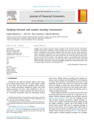
G. Baltussen, Z. Da, S. Lammers et al.Journal of Financial Economics 142 (2021) 377–403early as 30 minutes before close. This fits nicely into ourreasoning that rROD predicts rLH . Hedging demand on a particular LETF can be directly measured using its market capitalization and leverage and this hedging demand variesconsiderably in the cross-section and over time. We findstrong cross-sectional and time-series evidence that LETFs’hedging demand on a particular index drives the magnitude of its market intraday momentum pattern.What’s so special about the end of a trading day? Whilewe do find evidence that large price jumps during the daypredict subsequent returns, consistent with intraday hedging activities, the bulk of the hedge seems to take placetowards the end of the day. We conjecture that there areat least five reasons for this decision. First, from a theoretical point of view, Clewlow and Hodges (1997) show that, inthe presence of partially fixed transaction cost, it is optimalto hedge only partially after a large price movement, implying that additional hedging is required afterwards. Second, the additional hedging could be deferred to the endof the trading day for liquidity reasons. The U-shape intraday volume pattern across the equity, bond, commodity, and currency markets in Fig. 1 confirms that liquiditytends to be high right after open and before close. Further,spreads are generally lower and market depth higher whentrading towards the close. This is another reason why investors may not fully hedge their positions immediately after a jump during the day and will leave the bulk of hedging to be done in the last half hour, when liquidity is generally better, especially for trading larger quantities.Third, while hedging is partial during the day, it tendsto be complete at the end of the day to protect againstovernight risk. Brock and Kleidon (1992) and Hong andWang (20 0 0) show that lower liquidity and higher pricerisk overnight makes it optimal for market makers to closedelta positions before overnight. Fourth, holding positionsovernight typically incurs higher capital needs and investment frictions. For example, Bank for International Settlements (BIS) capital requirements are driven by deltas atclose. Further, margin requirements generally increase forovernight positions, while lending fees and margin interest are typically charged only on positions held overnight(Bogousslavsky, 2020). As a consequence, holding risky positions overnight not only comes with higher price risks,but also with higher capital requirements. Market participants therefore have an incentive to reduce delta at theend of the day to free up capital and save cost. Finally, aswe have demonstrated, market makers of index productssuch as LETFs have little choice but to hedge at the end ofthe day.3Besides hedging demand, other factors couldalso contribute to the market intraday momentum.Gao et al. (2018) discuss two: infrequent portfolio rebalancing and late informed trading. Under the infrequentrebalancing explanation, some institutional investors effectively choose to rebalance their portfolios in the firsthalf hour and others in the last half hour. Rebalancing inthe same direction can thus generate momentum intraday.Under the late informed trading explanation, traders whoare informed late trade in the last 30 minutes. Hence,the same information is incorporated into prices duringboth the first and the last 30 minutes, resulting in momentum. Both explanations hinge on the strong U-shapedintraday trading volume pattern, as informed trading andrebalancing are expected to primarily take place at thestart and end of the trading session, when liquidity is high(Admati and Pfleiderer, 1988; Bogousslavsky, 2016). Thefact that rROD better predicts rLH than rONF H suggests thatreturns during the day also matter, and that hedging is animportant driver of market intraday momentum.We conduct two additional tests that further differentiate hedging demand from informed trading. We first noticethat under the hedging explanation, the predictability ofrLH reflects transitory price pressure and should thereforebe reverted in the future. In contrast, the informed tradingexplanation builds upon the arrival of fundamental information, which should cause permanent price impact, andhence no reversal in predictability. Empirically, in all fourasset classes, returns in the next three days are opposite tothose of rLH . For equities, bonds, and commodities, there isa highly significant mean-reversion, consistent with transitory price pressure, which arises from hedging.For another piece of evidence supporting the hedgingchannel instead of informed trading, we turn to the underlying market for S&P 500, which closes at 4pm ET, at whichtime most related options and levered ETFs also settle. Yetfutures contracts on the S&P 500 index still trade activelyat substantial volume for another 15 minutes until the futures settles at 4:15pm ET, so informed trading at sufficientliquidity can well take place after 4pm ET. We find that thereturn predictability of rROD does not extend to the futuresreturn beyond 4pm ET, which seems hard to reconcile withthe informed trading channel.Our paper contributes to the voluminous literature onreturn momentum. In the cross-section, winners in thepast six months to one year earn higher returns up toone year in the future (see Jegadeesh and Titman, 1993,among others). Similarly in the time series, the past oneyear returns of an asset positively predict its future returns across many asset classes (see Moskowitz et al., 2012,among others). Instead, we focus on market momentumwithin a trading day. In this regard, our paper is mostclosely related to Gao et al. (2018) but differs in severalaspects. Our analysis is much more comprehensive in itscoverage, spanning indices and futures contracts across allmajor asset classes between 1974 and 2020. The market intraday momentum effect we observe is also different fromtheirs. And, most importantly, we discover a novel underlying economic force, which seems to be increasingly prominent. In a related study Elaut et al. (2018) show intraday momentum in the RUB/USD currency pair since 2005,which they attribute to dealers closing positions overnight.Our paper also relates to a growing literature on intraday price patterns. Recently, Lou et al. (2019) reportedstrong overnight and intraday return continuation and anoffsetting cross-period reversal at the individual stock leveland in equity return factors (see also Bogousslavsky, 2020;Hendershott et al., 2020). Muravyev and Ni (2019) andGoyenko and Zhang (2019) observe strong intraday and3The same holds for market makers of variance swaps, as payoff of avariance swap is calculated based on the closing levels of the underlyingindex.379

G. Baltussen, Z. Da, S. Lammers et al.Journal of Financial Economics 142 (2021) 377–403Fig. 1. Trading volume distribution during the day. This figure shows the average trading volume as a fraction of total daily volume per time bucket foreach asset class. The time buckets are (1) the “first half an hour” (F H, the first 30 minutes after the market open), (2) the “middle of the day” (M, from theend of F H to an hour before the market close), (3) the “second-to-last half an hour” (SLH, the second-to-last 30 minute interval), and (4) the “last half anhour” (LH, the last 30 minutes before the market close). Since bucket M contains more than 30 minutes, we divide its volume by the number of minutesin the bucket and multiply by 30, such that all buckets represent volume per 30 minutes. Per market, we divide the buckets’ volumes by the daily volumeand average over time to get the average volume fractions per market. For each asset class, we then take the average over the markets belonging to thatasset class. Shown are the results for equity index futures (Panel (a)), government bond futures (Panel (b)), commodity futures (Panel (c)), and currencyfutures (Panel (d)). Samples range from July 2003 to May 2020.overnight differences in option returns. In subsequentwork, Barbon and Buraschi (2020) show that gamma hedging also drives intraday momentum and reversal patternsin individual stocks throughout the trading day. Further,Heston et al. (2010) find evidence of intraday return seasonality in the cross-section of stocks: returns continueduring the same half-hour intervals as in previous trading days, lasting from 1 to up to 40 trading days. Whilethese studies focus on individual stocks and their options,our paper focuses on indices across a broad range of assetclasses.4 We also find market intraday momentum to bedistinct from intraday return seasonality, with rROD continuing to predict rLH even after controlling for rLH from previous days.4In addition, several studiesine intraday volatility (Chang etity estimators. Examples includeVan Dijk (2007), and Bollerslev etOur results reveal that hedging demand coming fromoptions and LETFs amplifies price changes and affects market return dynamics over several days. Several other recentstudies link the rise in indexing products (like ETFs) to sideeffects such as the amplification of fundamental shocks(Hong et al., 2012), excessive co-movement (Barberis et al.,20 05; Greenwood, 20 05; Greenwood, 20 08; Da and Shive,2018), a deterioration of the firm’s information environment (Israeli et al., 2017), increased non-fundamentalvolatility in individual stocks (Ben-David et al., 2018) andVIX and commodity futures markets (Todorov, 2019), andnon-fundamental shocks at the market level that resultin price reversals (Baltussen et al., 2019). Intraday gammahedging demand effects could contribute to short-termnegative market reversals shown in the latter paper. Ina related study, Bogousslavsky and Muravyev (2019) argue that an increase in indexing is associated with an increase in market close volumes and distortions in closingprice. These results are broadly consistent with the view inutilize intraday price data to examal., 1995) or the efficiency of volatilBollerslev et al. (20 0 0), Martens andal. (2018).380

G. Baltussen, Z. Da, S. Lammers et al.Journal of Financial Economics 142 (2021) 377–403Wurgler (2011) that indexing can affect the general properties of markets.The rest of the paper is organized as follows.Section 2 describes our data and provides summary statistics. Section 3 presents the main stylized facts about themarket intraday momentum pattern across the variousasset classes. Section 4 offers evidence supporting thegamma hedging demand channel. Section 5 concludes. TheAppendix contains additional descriptions of the data andvarious robustness results.nearly round-the-clock, but most of the trading happensduring the hours the underlying is trading. Trading volumeoutside of these hours is typically substantially lower. Bycontrast, the highest levels of trading volume clearly happen around open and close of the underlying equity index.As equity markets have clear trading hours, it is straightforward to select the trading hours of the equity index itself. We correct for changes in trading hours over our sample, as, for example, the S&P 500 opened 30 minutes laterbefore 1985.6For futures on non-equity assets, it is not that straightforward to select the trading hours, as, for example, government bonds are generally traded over the counter. Following the patterns in equity markets, we select tradinghours of government bond futures based on volume plotsand selecting “open” and “close” times based on spikes involume. These spikes consistently happen at preset times,signaling their suitability as opening and closing times. Forall but Australian and Japanese bond futures, this results inusing the regular opening hours of the futures as open, andthe end of the daily settlement period as close. We use theregular trading hours of Australian and Japanese futures astrading hours.The currency futures we use are all U.S. listed. Thesefutures show volume spikes at 8:21 and 15:00, which correspond to the open outcry hours of options on those futures; 15:00 also happens to be the end of the daily settlement period for these futures.The commodity futures in our sample have been subject to several changes in trading hours. Nowadays, mostof these futures trade almost 24 hours a day, but this usedto be different. Before the futures traded continuously, weconsider the actual trading hours of the futures as ourtrading hours. After the introduction of continuous trading, we select trading hours based on volume plots, as isthe practice for government bond futures and currency futures.For each of the asset classes, a more detailed description of the sample, along with trading hours at the end ofour sample, can be found in Appendix A. The trading hourswe consider over time and average volume plots are available upon request.To examine the presence of intraday return predictability, we calculate the return of buying at previous day’s(t 1) close (c) and selling 30 minutes after today’s (t)opening (o) for each futures or index,2. DataTo examine intraday momentum effects, we collect datafor the world’s largest, best traded, and most importantstock and government bond futures or indices in developedmarkets around the world, as well as for commodity, andcurrency futures. We obtain historical tick-by-tick data onthe major equity index, government bond, commodity andcurrency futures from Tick Data LLC5 The data consists of17 developed markets’ equity futures (6 North American, 8European, 3 Asian or Australian), 12 of which are also covered by data on their underlying equity indices; 16 developed markets bond futures (6 North American, 7 European,3 Asian or Australian); 21 commodity futures (5 metals, 4energies, 12 softs); and 8 currency futures with the sampleperiod ranging from December 1974 to May 2020.We retrieve one-minute intervals containing the corresponding open price, close price and trade volume. Volumedata is available from 2003 onwards. We consider the mostliquid contract (generally the nearest-to-delivery contract)and roll it over when the daily tick volume of the nextback-month contract exceeds the current contract. Following the procedure for intraday data filtering in BarndorffNielsen et al. (2008), we filter the data by subsequently(i) removing all observations with non-positive prices, (ii)removing all non-business days, (iii) removing all days inwhich the exchange closed earlier (such as Memorial Day),and (iv) removing all days in which the total traded volume is less than 100 contracts. This procedure ensures thatthe sample consists of regular trading days. Appendix Aprovides a detailed overview of the included futures contracts.To determine ON, FH, M, SLH, and LH hours, we establish the opening and closing times of markets using thefollowing procedure. We select the observations that correspond to the “common” trading hours of the market (i.e.,the openings hours of the cash (and ETF) market in linewith Gao et al. (2018)), which typically differ from futures’ trading hours (futures trade for extended time periods, nowadays often close to 24 hours a day). Our motivation for this choice is that futures are derivatives andare expected to behave like their underlying instruments;these are the moments at which positions are most likelyrebalanced. This corresponds to the trading hours of theunderlying for equity futures; e.g., we select the observations of the S&P E-Mini between 09:30 and 16:00, as theseare the trading hours of the S&P 500. Futures are traded5rONF H,t Po 30,t 1,Pc,t 1(1)and every following half-hour return until close.We argue that the return until the last half hour, the return of buying at previous day’s close and selling 30 minutes before today’s close,rROD,t Pc 30,t 1,Pc,t 1(2)6For several equity index futures, the standard contracts were quicklyoutgrown in terms of traded volume by their mini versions. To obtain thelargest sample, we first consider the standard contracts and replace themwith the mini versions after its introduction.www.tickdata.com.381

G. Baltussen, Z. Da, S. Lammers et al.Journal of Financial Economics 142 (2021) 377–403predicts the last half-hour return. To investigate the addedvalue of considering the return until the last half hour overthe first half-hour return, we also consider the return between the end of the first half hour and the last hour andthe second-to-last half hour,rM,t Pc 60,t 1Po 30,trSLH,t Pc 30,t 1.Pc 60,twindow, requiring at least 500 observations, or about twoyears of data.We then define the OOS R2 as follows: T(rLH,t rˆLH,t )2R2OOS 1 t 1,T2t 1 (rLH,t r̄LH,t )(3)where rˆLH,t is the predicted last half-hour return on day tand r̄LH,t is the historical average last half-hour return untilt 1 (expanding window).To see whether the MSPE is significantly lower than using the recursive historical mean, we perform a Clark andWest (2007) test. First, define ft ,(4)We remove all observations outside of the trading hourswe consider a trading day. This way, the overnight return,which is contained in the first half-hour return, is computed using the price at our closing time on the previousday: e.g., a German future usually trades between 08:00and 22:00. When adjusting the time frame to 08:00–17:15,rONF H is computed over the closing price at 17:15 yesterdayand the closing price of the first half hour today, 08:30.For each asset class, we construct various groups, oneof which contains all futures belonging to that asset class.Within equity index and bond futures, we consider geographical groups for U.S.-based futures (“USA”), futuresfrom Europe (“EU”), and futures from Australia or Asia(“Australasia”). Commodity futures are not country specific,such that we consider categorical groups for metals, energies, and softs.Table 1 lists the tickers and trading hours for all thefutures contracts we used in the paper.ft (rLH,t r̄LH,t )2 ((rLH,t rˆLH,t )2 (r̄LH,t rˆLH,t )2 ),(9)and the test statistic follows from regressing ft on a constant. A significant positive constant implies that predictor rˆLH,t , the first half-hour return or return until the lasthalf hour before close, results in a significantly lower MSPEthan when using r̄LH,t , the recursive historical mean.3.1. Baseline resultsIn our analyses, we first pool together futures contractsin the same asset class and the regressions’ results are provided in Table 2. Panels A through D report the resultsfor equity, bond, commodity, and currency futures, respectively.To the best of our knowledge, there is no pooled outof-sample R2 measure, so we define a measure that represents a pooled OOS R2 . Define Ft as the futures availableat day t and n(Ft ) the number of futures available on dayt. We define rLH, f,t as the last half-hour return for futuref Ft on day t, rˆLH, f,t our prediction for the last half hour,and r̄LH, f,t the historical average last half-hour return untilt 1. Then, R2OOS is defined as:3. Market intraday momentum everywhereIn this section, we show a robust market intraday momentum effect in all four asset classes we examine.We consider several regression specifications for predicting the last half-an-hour return(rLH ). In the first specification, the only predictor is the return from previousclose to the end of the first half an hour (rONF H ), as inGao et al. (2018):rLH,t α βONF H · rONF H,t εt . TR2OOS 1 t 1 Tt 1(5) f Ft f Ft(rLH, f,t ˆrLH, f,t )2n(Ft )(rLH, f,t r̄LH, f,t )2.(10)n(Ft )Gao et al. (2018) examine for ten equity ETFs and onebond ETF how the return in each of the 30-minute intervals during the day predicts the return in the last halfan hour. They find rONF H to have the strongest predictivepower, followed by rSLH . Panel A of Table 2 confirms thispattern in an extended sample period and across differentstock markets. Column (1) finds a strong predictive powerin rONF H on a stand-alone basis. Column (2) presents theresults for Eq. (6); rONF H is again highly significant (t-value 6.46), followed by rSLH (t-value 4.82). Interestingly, thereturns in other 30-minute intervals, when combined intoone rM variable, are also significant in predicting rLH (tvalue 4.43). In other words, all returns during the day(prior to the last half an hour) have predictive power onrLH .In Column (3) of Panel A, we find that combining allreturns during the day (prior to the last half an hour)into rROD generates the strongest predictive power. First,rROD has the highest t-value, 7.29. In addition, rROD has thehighest out-of-sample R-squared (R2OOS ), 2.88%. In contrast,In the second specification, we consider multiple predictors. In addition to rONF H , we also include the returnduring the middle of the day (rM ) and the return in thesecond-to-last half an hour (rSLH ):rLH,t α βONF H · rONF H,t βM · rM,t βSLH · rSLH,t εt .(6)In the third specification, we combine the returns fromall three periods into the return during the rest of the day(rROD ):rLH,t α βROD · rROD,t εt .(8)(7)We

To facilitate our discussion, we define a trading day as the 24-hour period from the market close on day t 1 to the market close on day t. We select the open and close time to match the "common" trading hours of the market. The time line below then partitions the trading day into five parts: overnight (ON, from close to open);