Transcription
In- ttaDomik,UniversityofPaderborn,GermanyAbstract: We are describing two exercises to deepen the understanding of two popular real-time shadowalgorithms, namely shadow mapping and shadow volumes. Each of the exercises takes less than 10 minutes toperform during lecture time and leads to a profounder understanding and serves as a basis for further discussionsof improvements of these algorithms. By using this exercise we noticed an evident increase in implementingshadow algorithms for later real-time graphics projects.1. BackgroundofCourseThe course “Computer Graphics Rendering” at the Computer Science Department atthe University of Paderborn is for advanced Bachelor students who already hadsome fundamental Computer Graphics course or are quick learners. This renderingcourse emphasizes Shader programming and finishes with group projects in real-timerendering. As a basis for teaching this course the lecturer uses the books [AHH11]and [L12], and takes background and ideas from [AS12] and [BC12]. Shadowalgorithms are discussed in one 1.5 hour lecture together with other globalillumination topics for real-time rendering (such as caustics and ambient occlusion),so time is limited and should be used well. Because a profound understanding ofalgorithm and math underlying a real-time graphics implementation is of essence tous, we stop each lecture for one or two suitable In-Class exercises. It took us somethought to invent two short In-Class Exercises for Shadow algorithms – thus wedecided to share these with the community.2.In- ‐ClassExerciseforShadowMappingAlgorithmsThis exercise (ShadowMapExercise.pdf) can be downloaded from www.unipaderborn.de/cs/vis. Here is a step-by-step explanation.The Shadow Mapping algorithm has been proposed first by Williams [W78]. In thelecture, we use a modern description of the algorithm as it follows the books [AHH11]or [L12]. The idea is based on the fact that –considering one ray of light - objectpoints in shadow are farther away from the light source than illuminated object points.Setting the viewpoint of a camera into the light position, all visible object points are litand non-visible object points are in shadow. We store the distances between the lightsource and visible points (from the light source) in an array (called “shadow map”) forlater use. From the view of the camera, for each visible object point (such as verticesva and vb in Figure 1) we can calculate the distance to the light source and compare itto the recovered distance value stored in our array. As we can see in Figure 1, thedistance for object point va to the light source will be the same as recovered in theshadow map. The distance for object point vb will be longer than the value recoveredfrom the shadow map, indicating that it is in shadow. Let us use this idea for thefollowing procedure and accompany it with the first In-Class exercise:
Figure 1. Basic idea of Shadow Mapping: The shadow map z contains distances from object points to light source.Two vertices va and vb are seen from the camera. Vertex va has the same distance to the light source asrecovered from the shadow map at the corresponding location (s,t). Vertex vb has a longer distance to the lightsource than recovered from the shadow map at the corresponding location (s,t). The shadow mapping algorithmtherefore decides that vb is in shadow and va is not in shadow.First render the scene from the position of the light source. This results in theprojection of each object point p onto the near plane of the light using theModelViewProjection Matrix ML:M L p p L ( pxL , pyL , pzL )TOnly keep the content of the z-buffer and store it in a map ( shadow map). Everyother result of the rendering process, e.g. color buffer, is dispensable. Let’s take alook at this 2d shadow map and name it z(s,t): The shadow map z(s,t) now containsdepth values z ( distances between light source and lit object points) at each equallyspaced 2d location (s,t), where (s,t) describe the sampling rate of this renderingprocedure.
Figure 2. A cube is rendered from the view of the light source; the resulting content of the z-buffer is saved in a“shadow map”.For the set-up of Figure 2, students can fill one line of the shadow map z( at thevariousby looking up the distances from the near plane (relative to the light ulting in (or similar to):zt341Next render the scene from the position of the camera. This will result in filling thez-buffer ( distance between camera and visible object points) and the color buffer forour rendering process. We can calculate the distance from each visible point q to thelight source by usingS M L q q L (qxL , qyL , qzL )T(where S is a scaling matrix ensuring the correct scaling) and compare this distance(call it z’) with the previously stored z values in the shadow map. If the distancescorrespond, the visible point is lit, if the new value z’ is larger than z, point q is inshadow.
Figure 3. The cube is now rendered from the position of the camera. Object points visible from the camera areequally spaced in the corresponding image plane.The setup in Figure 3 shows eight equally spaced image/object locations (a . h)when rendering our cube. For one line of the current color buffer we fill in thedistances z’ from object point to light source by looking them up in Figure 3.z'abcdefghWe also have to remember the corresponding index t of the shadow map in relationto the new spacing in image (camera) lting in the following z’ values and corresponding shadow map index (locationst):z't234266297377546577608648Next compare the values z and z’ and make a shadow decision. Where z z’ weexpect lit points and where z z’ we expect shadow points for this indicates thatthere is another object point closer to the light source than the current object pointunder investigation.This final decision can be expressed by the Heaviside function
#% 1, for(z z') 0H (z(t) z') &% 0, for(z z') 0If H(z(t)-z’) 0 (or slightly larger than zero because of inaccuracies), then q lies inshadow, if H(z(t)-z’) is negative, q is lit.For the next two lines of exercise we compare z(t) and z’, but remember to use thecorresponding shadow map index t resulting inz(t) - z'Correspondingindex in imagebuffer (a h)Correspondingindex in shadowmap (t)Shadow decisionH(z(t)-z’)s(hadowed) orlit?-2a1b1c-7d-27 -27 2efg-2h4677678801100010slitlitssslitsComparing this result with Figure 3 we see that the decision is not correct for imageindex b and h. This phenomenon is called self-shadow aliasing and is treated in thenext section.Improvement of self-shadow aliasing. One can easily imagine that the precisecomparison of z and z’ leads to errors. Each z entry in the shadow map representsan area in object space whose size is dependent on the applied sampling rate duringthe first rendering from the light source. Depending on where p or where q arelocated within this area, the distance of q might be larger than the distance of p to thelight source and erroneously determine shadow for this location. This so called selfshadowing can be corrected by adding a constant bias to the entries of the shadowmap. Therefore allow students to add a constant bias c (e.g. c 2) to the entries of theshadow map, resulting in a comparison z(t) c-z'z(t) 2 - z'033-5-25 -25 401lit1lit0s0s1litand a new (correct) shadow decisionH(z(t) 2 - z')s(hadowed) orlit?1lit0s1litThe solution sheet (ShadowMapSolution.pdf) can also be downloaded from www.unipaderborn.de/cs/vis.
This exercise is easy to extend by other algorithm improvements, e.g. thepercentage-closer filtering [AHH11].3.In- ‐ClassExerciseforShadowVolumeAlgorithmsThis exercise (ShadowVolumesExercise.pdf) can be downloaded from www.unipaderborn.de/cs/vis. Here is the step-by-step explanation.The Shadow Volume Algorithm originates by Franklin Crow, 1977 [C77]. In thelecture, we use a modern description of the algorithm as it follows the books [AHH11]or [L12]. Modern hardware increases the speed of this algorithm so that it is now incommon use for dynamic real-time shadowing. The basic idea behind this algorithmis that the shadow of an object is constructed as a volume by extruding the object’ssilhouette (with respect to a light source) away from this light source (grey areaextruding from the green object in Figure 4).Figure 4. A light source lights a green object that will block out light for other objects within its “shadow volume”.(The shadow volumes for the orange and blue object are not drawn in this Figure.) A line of sight from the camerawill intersect a front facing polygon of the shadow volume when rendering a point on the blue object; a line of sightfrom the camera will intersect a front facing and a back facing polygon of the shadow volume when rendering apoint on the orange object. Intersecting (crossing) a front facing polygon adds one to the stencil buffer,intersecting a backfacing polygon subtracts one to the stencil buffer, leaving the stencil buffer with 1 for thecorresponding image location of the object point on the blue object and with 0 for the corresponding imagelocation of the object point on the orange object.Those parts of other objects lying inside this object’s shadow volume are in shadow.For a typical scene, many shadow volumes will exist. A ray of sight sent out from thecamera to an object point might cross a shadow volume's surface on entering andexiting the volume. When increasing a counter on entering and decreasing it onexiting the volume, the counter will have a non-zero value if the ray ends on ashadowed object. This procedure can be realized by (non-visibly) drawing thevolume's front and back faces and using the stencil-buffer as the counter.The classic algorithm called “z-pass Shadow Volume algorithm” consists of two parts:Part 1: initialize all buffers (including the stencil buffer) and render the scene asseen from the camera using only ambient illumination of the light source (this makesthe resulting color buffer look like a scene in full shadow). Keep the depth (z) buffer.
Part 2: Set the depth test to pass for z values smaller and equal values than in thedepth buffer. Now in a first pass render all the front faces of the shadow volumeswithout drawing to the color buffer or changing the depth buffer. Instead, this and thenext rendering pass will aid only in filling the stencil buffer. Whenever a depth test isperformed the stencil buffer is increased if the test is passed. Nothing happens if thedepth test fails.Figure 5. Two objects and their shadow volumes in front of a surface being rendered into the image buffer withimage locations a through e.Applying this procedure, students can use Figure 5 (a) to track the intersection of thecamera rays and the volume faces to determine the changes to the stencil buffer:Change in stencil buffer 2 2 1 1 1 at locationabcdeNow render the back faces in a second pass, and decrease the value in the stencilbuffer whenever the depth test is being passed. Again the changes to the stencilbuffer are recorded.Change in stencil buffer-1-1-100By summing up the changes the resulting state of the stencil can be computed.Content of stencil buffer11011Now in a final rendering pass of the objects in the scene (where only fragments withstencil value 0 are being lit) renders the scene correctly. From the stencil buffer thestudents can derive the shadow decision for each pixel.s(hadowed) or lit?sslitssThis works well when the camera is outside any shadow volume. When the camera'snear plane intersects the shadow volume, this algorithm fails. The studentsreproduce this problem by repeating the algorithm using a slightly changed cameraposition (Figure 5 b) and observe the wrong results in the final shadow decision:Change after front face11000
renderingChange after back facerendering-1-1-100Resulting stencil buffer00-100s(hadowed) or lit?litlitslitlitChanges to the original “z-pass” algorithm lead to a camera position robust solution,called the “z-fail Shadow Volume algorithm”. A robust solution [EK03] demandsseveral changes in the approach: first, the silhouette's extrusion has to be changed toextrude the vertices (mathematically) onto the camera's far plane, by using a specialprojection matrix. This ensures that all normal geometry resides inside the shadowvolume. Second, a cap for the shadow volume has to be added onto the back face –and front face! For our example, Figure 6 points out the relevant front faces, backfaces and back face cap.Figure 6. For the Z-Fail algorithm, the silhouette's extrusion has to be changed to include a cap at the end of theshadow volume. This figure emphasizes the relevant front faces (f”), back faces and back caps (“b”) for renderinga surface from the camera’s point of view.Also the drawing decision and the stencil operation have to be changed to thefollowing:Part 1: initialize all buffers (including the stencil buffer) and render the scene asseen from the camera using only ambient illumination of the light source. Keep thedepth (z) buffer.Part 2: Set the depth test to pass for z values smaller than in the depth buffer. Now ina first pass render the front faces of the shadow volumes without drawing to thecolor buffer or changing the depth buffer. Whenever a depth test is performed thestencil buffer is decreased if the test fails. Again, the changes can be tracked bychecking the camera ray in Figure 5(c). This time, however, the scene behind thevisible geometry has to be considered, resulting inChange in stencil buffer 00-100
at locationabcdeNow render the back faces in a second pass, and increase the value in the stencilbuffer whenever the depth test fails.Change in stencil buffer 1 1 1 1 1The resulting stencil buffer and shadow decision demonstrate how the z-fail methodsolves the preceding problems.Content of stencil buffer11011s(hadowed) or l(it)?sslitssThe solution sheet (ShadowVolumesSolution.pdf) can also be downloaded ts produce a final (group) project for this course, where they are free toconstruct an animation of a virtual world of their choice and making. They are beinggraded for the real-time visual effects they implement and the models they generatefor their world. They are free to use additionally imported models to fill their world asthey see suited. In 2012 we had 19 students submitting 6 projects (with roughly 3students per group), only one project group implemented a shadow algorithm; in2013 we had 8 group projects, again only one project included a shadow algorithm;in 2014 (when we implemented the In-Class shadow exercises) we had 26 projects,where 10 projects implemented a real-time shadow algorithm.Over the last years we have submitted the best of the group projects resulting fromthis course to ACM SIGGRAPH’s “Faculty Submitted Student Work” Competition.The following two snapshots (Figure 7 and Figure 8) are from such submittedanimations.
Figure 7: Student group project “The End of the World” showing shadow of moving ball next to many other realtime effects, such as blooming or particle systems.Figure 8: Student group project “Sheep at a Picnic” showing a candle flame throwing shadows of objects on table.Acknowledgement: Peter Wagener, Stanislaw Eppinger, Tobias Rojahn, ThomasLöcke, Kathlén Kohn for their projects; Stephan Arens as Lab coordinator; MikeBailey and Scott Owen for Review.References[AHH11] Tomas Akenine-Möller, Eric Haines and Naty Hoffman, Real-TimeRendering, Third Edition. Boca Raton, FL, Taylor & Francis, 2011.
[AS12] Edward, Angel and Dave Shreiner, Interactive Computer Graphics: A Topdown Approach with Shader-based OpenGL, 6. Boston, MA, Addison-Wesley, 2012.[BC12] Mike Bailey and Steve Cunningham, Graphics Shaders: Theory and Practice,2nd. Boca Raton, FL, Taylor & Francis, 2012.[C77] Franklin C. Crow. 1977. Shadow algorithms for computer graphics inProceedings of the 4th annual conference on Computer graphics and interactivetechniques (SIGGRAPH '77). New York, NY, ACM, 1977, pp. 242-248.[EK03] Cass Everitt and Mark J. Kilgard (2003), Practical and robust stenciledshadow volumes for hardware-accelerated rendering. In: arXiv:cs/0301002[L12] Eric Lengyel, Mathematics for 3D Game Programming and ComputerGraphics, Third Edition. Boston, MA, Cengage Learning, 2012.[W78] Lance Williams. 1978. Casting curved shadows on curved surfaces inProceedings of the 5th annual conference on Computer graphics and interactivetechniques (SIGGRAPH '78). New York, NY, ACM, pp. 270-274.
(The shadow volumes for the orange and blue object are not drawn in this Figure.) A line of sight from the camera will intersect a front facing polygon of the shadow volume when rendering a point on the blue object; a line of sight from the camera will intersect a front facing and a back facing polyg