Transcription
INTRODUCTION toSTRING FIELD THEORYWarren SiegelUniversity of MarylandCollege Park, MarylandPresent address: State University of New York, Stony /insti.physics.sunysb.edu/ siegel/plan.html
CONTENTSPreface1. Introduction1.1. Motivation11.2. Known models (interacting) 31.3. Aspects41.4. Outline62. General light cone2.1. Actions82.2. Conformal algebra102.3. Poincaré algebra132.4. Interactions162.5. Graphs192.6. Covariantized light cone20Exercises233. General BRST3.1. Gauge invariance andconstraints253.2. IGL(1)293.3. OSp(1,1 2)353.4. From the light cone383.5. Fermions453.6. More dimensions46Exercises514. General gauge theories4.1. OSp(1,1 2)524.2. IGL(1)624.3. Extra modes674.4. Gauge fixing684.5. Fermions75Exercises795. Particle5.1. Bosonic815.2. BRST845.3. Spinning865.4. Supersymmetric955.5. SuperBRST110Exercises1186. Classical mechanics6.1. Gauge covariant6.2. Conformal gauge6.3. Light coneExercises7. Light-cone quantum mechanics7.1. Bosonic7.2. Spinning7.3. SupersymmetricExercises8. BRST quantum mechanics8.1. IGL(1)8.2. OSp(1,1 2)8.3. Lorentz gaugeExercises9. Graphs9.1. External fields9.2. Trees9.3. LoopsExercises10. Light-cone field theoryExercises11. BRST field theory11.1. Closed strings11.2. ComponentsExercises12. Gauge-invariant interactions12.1. Introduction12.2. Midpoint 5217228230241
PREFACEFirst, I’d like to explain the title of this book. I always hated books whose titlesbegan “Introduction to.” In particular, when I was a grad student, books titled“Introduction to Quantum Field Theory” were the most difficult and advanced textbooks available, and I always feared what a quantum field theory book which wasnot introductory would look like. There is now a standard reference on relativisticstring theory by Green, Schwarz, and Witten, Superstring Theory [0.1], which consists of two volumes, is over 1,000 pages long, and yet admits to having some majoromissions. Now that I see, from an author’s point of view, how much effort is necessary to produce a non-introductory text, the words “Introduction to” take a moretranquilizing character. (I have worked on a one-volume, non-introductory text onanother topic, but that was in association with three coauthors.) Furthermore, thesewords leave me the option of omitting topics which I don’t understand, or at leastbeing more heuristic in the areas which I haven’t studied in detail yet.The rest of the title is “String Field Theory.” This is the newest approachto string theory, although the older approaches are continuously developing newtwists and improvements. The main alternative approach is the quantum -string-picture/Polyakov/conformal- “fieldtheory”) one, which necessarily treats a fixed number of fields, corresponding tohomogeneous equations in the field theory. (For example, there is no analog in themechanics approach of even the nonabelian gauge transformation of the field theory,which includes such fundamental concepts as general coordinate invariance.) It is alsoan S-matrix approach, and can thus calculate only quantities which are gauge-fixed(although limited background-field techniques allow the calculation of 1-loop effectiveactions with only some coefficients gauge-dependent). In the old S-matrix approachto field theory, the basic idea was to start with the S-matrix, and then analyticallycontinue to obtain quantities which are off-shell (and perhaps in more general gauges).However, in the long run, it turned out to be more practical to work directly withfield theory Lagrangians, even for semiclassical results such as spontaneous symmetrybreaking and instantons, which change the meaning of “on-shell” by redefining thevacuum to be a state which is not as obvious from looking at the unphysical-vacuumS-matrix. Of course, S-matrix methods are always valuable for perturbation theory,
but even in perturbation theory it is far more convenient to start with the field theoryin order to determine which vacuum to perturb about, which gauges to use, and whatpower-counting rules can be used to determine divergence structure without specificS-matrix calculations. (More details on this comparison are in the Introduction.)Unfortunately, string field theory is in a rather primitive state right now, and noteven close to being as well understood as ordinary (particle) field theory. Of course,this is exactly the reason why the present is the best time to do research in this area.(Anyone who can honestly say, “I’ll learn it when it’s better understood,” should marka date on his calendar for returning to graduate school.) It is therefore simultaneouslythe best time for someone to read a book on the topic and the worst time for someoneto write one. I have tried to compensate for this problem somewhat by expanding onthe more introductory parts of the topic. Several of the early chapters are actuallyon the topic of general (particle/string) field theory, but explained from a new pointof view resulting from insights gained from string field theory. (A more standardcourse on quantum field theory is assumed as a prerequisite.) This includes the useof a universal method for treating free field theories, which allows the derivation ofa single, simple, free, local, Poincaré-invariant, gauge-invariant action that can beapplied directly to any field. (Previously, only some special cases had been treated,and each in a different way.) As a result, even though the fact that I have tried tomake this book self-contained with regard to string theory in general means that thereis significant overlap with other treatments, within this overlap the approaches aresometimes quite different, and perhaps in some ways complementary. (The treatmentsof ref. [0.2] are also quite different, but for quite different reasons.)Exercises are given at the end of each chapter (except the introduction) to guidethe reader to examples which illustrate the ideas in the chapter, and to encouragehim to perform calculations which have been omitted to avoid making the length ofthis book diverge.This work was done at the University of Maryland, with partial support fromthe National Science Foundation. It is partly based on courses I gave in the falls of1985 and 1986. I received valuable comments from Aleksandar Miković, ChristianPreitschopf, Anton van de Ven, and Harold Mark Weiser. I especially thank BartonZwiebach, who collaborated with me on most of the work on which this book wasbased.June 16, 1988Originally published 1988 by World Scientific Publishing Co Pte Ltd.ISBN 9971-50-731-5, 9971-50-731-3 (pbk)July 11, 2001: liberated, corrected, bookmarks added (to pdf)Warren Siegel
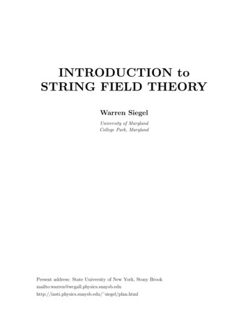
1.1. Motivation11. INTRODUCTION1.1. MotivationThe experiments which gave us quantum theory and general relativity are nowquite old, but a satisfactory theory which is consistent with both of them has yetto be found. Although the importance of such a theory is undeniable, the urgencyof finding it may not be so obvious, since the quantum effects of gravity are notyet accessible to experiment. However, recent progress in the problem has indicatedthat the restrictions imposed by quantum mechanics on a field theory of gravitationare so stringent as to require that it also be a unified theory of all interactions, andthus quantum gravity would lead to predictions for other interactions which can besubjected to present-day experiment. Such indications were given by supergravitytheories [1.1], where finiteness was found at some higher-order loops as a consequenceof supersymmetry, which requires the presence of matter fields whose quantum effectscancel the ultraviolet divergences of the graviton field. Thus, quantum consistency ledto higher symmetry which in turn led to unification. However, even this symmetry wasfound insufficient to guarantee finiteness at all loops [1.2] (unless perhaps the gravitonwere found to be a bound-state of a truly finite theory). Interest then returned totheories which had already presented the possibility of consistent quantum gravitytheories as a consequence of even larger (hidden) symmetries: theories of relativisticstrings [1.3-5]. Strings thus offer a possibility of consistently describing all of nature.However, even if strings eventually turn out to disagree with nature, or to be toointractable to be useful for phenomenological applications, they are still the onlyconsistent toy models of quantum gravity (especially for the theory of the gravitonas a bound state), so their study will still be useful for discovering new properties ofquantum gravity.The fundamental difference between a particle and a string is that a particle is a 0dimensional object in space, with a 1-dimensional world-line describing its trajectoryin spacetime, while a string is a (finite, open or closed) 1-dimensional object in space,which sweeps out a 2-dimensional world-sheet as it propagates through spacetime:
21. INTRODUCTIONxparticlerX(σ)stringx(τ )X(σ, τ he nontrivial topology of the coordinates describes interactions. A string can beeither open or closed, depending on whether it has 2 free ends (its boundary) or isa continuous ring (no boundary), respectively. The corresponding spacetime figureis then either a sheet or a tube (and their combinations, and topologically morecomplicated structures, when they interact).Strings were originally intended to describe hadrons directly, since the observedspectrum and high-energy behavior of hadrons (linearly rising Regge trajectories,which in a perturbative framework implies the property of hadronic duality) seemsrealizable only in a string framework. After a quark structure for hadrons becamegenerally accepted, it was shown that confinement would naturally lead to a stringformulation of hadrons, since the topological expansion which follows from using1/N color as a perturbation parameter (the only dimensionless one in massless QCD,besides 1/N f lavor ), after summation in the other parameter (the gluon coupling, whichbecomes the hadronic mass scale after dimensional transmutation), is the same per-
1.2. Known models (interacting)3turbation expansion as occurs in theories of fundamental strings [1.6]. Certain stringtheories can thus be considered alternative and equivalent formulations of QCD, justas general field theories can be equivalently formulated either in terms of “fundamental” particles or in terms of the particles which arise as bound states. However,in practice certain criteria, in particular renormalizability, can be simply formulatedonly in one formalism: For example, QCD is easier to use than a theory where gluonsare treated as bound states of self-interacting quarks, the latter being a nonrenormalizable theory which needs an unwieldy criterion (“asymptotic safety” [1.7]) torestrict the available infinite number of couplings to a finite subset. On the otherhand, atomic physics is easier to use as a theory of electrons, nuclei, and photonsthan a formulation in terms of fields describing self-interacting atoms whose excitations lie on Regge trajectories (particularly since QED is not confining). Thus,the choice of formulation is dependent on the dynamics of the particular theory, andperhaps even on the region in momentum space for that particular application: perhaps quarks for large transverse momenta and strings for small. In particular, therunning of the gluon coupling may lead to nonrenormalizability problems for smalltransverse momenta [1.8] (where an infinite number of arbitrary couplings may showup as nonperturbative vacuum values of operators of arbitrarily high dimension), andthus QCD may be best considered as an effective theory at large transverse momenta(in the same way as a perturbatively nonrenormalizable theory at low energies, likethe Fermi theory of weak interactions, unless asymptotic safety is applied). Hence, astring formulation, where mesons are the fundamental fields (and baryons appear asskyrmeon-type solitons [1.9]) may be unavoidable. Thus, strings may be importantfor hadronic physics as well as for gravity and unified theories; however, the presentlyknown string models seem to apply only to the latter, since they contain masslessparticles and have (maximum) spacetime dimension D 10 (whereas confinement inQCD occurs for D 4).1.2. Known models (interacting)Although many string theories have been invented which are consistent at thetree level, most have problems at the one-loop level. (There are also theories whichare already so complicated at the free level that the interacting theories have beentoo difficult to formulate to test at the one-loop level, and these will not be discussedhere.) These one-loop problems generally show up as anomalies. It turns out thatthe anomaly-free theories are exactly the ones which are finite. Generally, topologi-
41. INTRODUCTIONcal arguments based on reparametrization invariance (the “stretchiness” of the stringworld sheet) show that any multiloop string graph can be represented as a tree graphwith many one-loop insertions [1.10], so all divergences should be representable as justone-loop divergences. The fact that one-loop divergences should generate overlappingdivergences then implies that one-loop divergences cause anomalies in reparametrization invariance, since the resultant multi-loop divergences are in conflict with theone-loop-insertion structure implied by the invariance. Therefore, finiteness shouldbe a necessary requirement for string theories (even purely bosonic ones) in order toavoid anomalies in reparametrization invariance. Furthermore, the absence of anomalies in such global transformations determines the dimension of spacetime, which inall known nonanomalous theories is D 10. (This is also known as the “critical,” ormaximum, dimension, since some of the dimensions can be compactified or otherwisemade unobservable, although the number of degrees of freedom is unchanged.)In fact, there are only four such theories:I:N 1 supersymmetry, SO(32) gauge group, open [1.11]IIA,B:N 2 nonchiral or chiral supersymmetry [1.12]heterotic: N 1 supersymmetry, SO(32) or E8 E8 [1.13]or broken N 1 supersymmetry, SO(16) SO(16) [1.14]All except the first describe only closed strings; the first describes open strings, whichproduce closed strings as bound states. (There are also many cases of each of thesetheories due to the various possibilities for compactification of the extra dimensionsonto tori or other manifolds, including some which have tachyons.) However, for simplicity we will first consider certain inconsistent theories: the bosonic string, which hasglobal reparametrization anomalies unless D 26 (and for which the local anomaliesdescribed above even for D 26 have not yet been explicitly derived), and the spinning string, which is nonanomalous only when it is truncated to the above strings.The heterotic strings are actually closed strings for which modes propagating in theclockwise direction are nonsupersymmetric and 26-dimensional, while the counterclockwise ones are N 1 (perhaps-broken) supersymmetric and 10-dimensional, orvice versa.1.3. AspectsThere are several aspects of, or approaches to, string theory which can best beclassified by the spacetime dimension in which they work: D 2, 4, 6, 10. The 2D
1.3. Aspects5approach is the method of first-quantization in the two-dimensional world sheet sweptout by the string as it propagates, and is applicable solely to (second-quantized) perturbation theory, for which it is the only tractable method of calculation. Since itdiscusses only the properties of individual graphs, it can’t discuss properties whichinvolve an unfixed number of string fields: gauge transformations, spontaneous symmetry breaking, semiclassical solutions to the string field equations, etc. Also, it candescribe only the gauge-fixed theory, and only in a limited set of gauges. (However,by introducing external particle fields, a limited amount of information on the gaugeinvariant theory can be obtained.) Recently most of the effort in this area has beenconcentrated on applying this approach to higher loops. However, in particle fieldtheory, particularly for Yang-Mills, gravity, and supersymmetric theories (all of whichare contained in various string theories), significant (and sometimes indispensable)improvements in higher-loop calculations have required techniques using the gaugeinvariant field theory action. Since such techniques, whose string versions have notyet been derived, could drastically affect the S-matrix techniques of the 2D approach,we do not give the most recent details of the 2D approach here, but some of the basicideas, and the ones we suspect most likely to survive future reformulations, will bedescribed in chapters 6-9.The 4D approach is concerned with the phenomenological applications of thelow-energy effective theories obtained from the string theory. Since these theories arestill very tentative (and still too ambiguous for many applications), they will not bediscussed here. (See [1.15,0.1].)The 6D approach describes the compactifications (or equivalent eliminations) ofthe 6 additional dimensions which must shrink from sight in order to obtain theobserved dimensionality of the macroscopic world. Unfortunately, this approach hasseveral problems which inhibit a useful treatment in a book: (1) So far, no justificationhas been given as to why the compactification occurs to the desired models, or to4 dimensions, or at all; (2) the style of compactification (Ka luża-Klein, Calabi-Yau,toroidal, orbifold, fermionization, etc.) deemed most promising changes from yearto year; and (3) the string model chosen to compactify (see previous section) alsochanges every few years. Therefore, the 6D approach won’t be discussed here, either(see [1.16,0.1]).What is discussed here is primarily the 10D approach, or second quantization,which seeks to obtain a more systematic understanding of string theory that wouldallow treatment of nonperturbative as well as perturbative aspects, and describe the
61. INTRODUCTIONenlarged hidden gauge symmetries which give string theories their finiteness and otherunusual properties. In particular, it would be desirable to have a formalism in whichall the symmetries (gauge, Lorentz, spacetime supersymmetry) are manifest, finitenessfollows from simple power-counting rules, and all possible models (including possible4D models whose existence is implied by the 1/N expansion of QCD and hadronicduality) can be straightforwardly classified. In ordinary (particle) supersymmetricfield theories [1.17], such a formalism (superfields or superspace) has resulted in muchsimpler rules for constructing general actions, calculating quantum corrections (supergraphs), and explaining all finiteness properties (independent from, but verified by,explicit supergraph calculations). The finiteness results make use of the backgroundfield gauge, which can be defined only in a field theory formulation where all symmetries are manifest, and in this gauge divergence cancellations are automatic, requiringno explicit evaluation of integrals.1.4. OutlineString theory can be considered a particular kind of particle theory, in that itsmodes of excitation correspond to different particles. All these particles, which differin spin and other quantum numbers, are related by a symmetry which reflects theproperties of the string. As discussed above, quantum field theory is the most complete framework within which to study the properties of particles. Not only is thisframework not yet well understood for strings, but the study of string field theory hasbrought attention to aspects which are not well understood even for general types ofparticles. (This is another respect in which the study of strings resembles the studyof supersymmetry.) We therefore devote chapts. 2-4 to a general study of field theory.Rather than trying to describe strings in the language of old quantum field theory,we recast the formalism of field theory in a mold prescribed by techniques learnedfrom the study of strings. This language clarifies the relationship between physicalstates and gauge degrees of freedom, as well as giving a general and straightforwardmethod for writing free actions for arbitrary theories.In chapts. 5-6 we discuss the mechanics of the particle and string. As mentionedabove, this approach is a useful calculational tool for evaluating graphs in perturbation theory, including the interaction vertices themselves. The quantum mechanicsof the string is developed in chapts. 7-8, but it is primarily discussed directly as anoperator algebra for the field theory, although it follows from quantization of the classical mechanics of the previous chapter, and vice versa. In general, the procedure of
1.4. Outline7first-quantization of a relativistic system serves only to identify its constraint algebra,which directly corresponds to both the field equations and gauge transformations ofthe free field theory. However, as described in chapts. 2-4, such a first-quantizationprocedure does not exist for general particle theories, but the constraint system canbe derived by other means. The free gauge-covariant theory then follows in a straightforward way. String perturbation theory is discussed in chapt. 9.Finally, the methods of chapts. 2-4 are applied to strings in chapts. 10-12, wherestring field theory is discussed. These chapters are still rather introductory, sincemany problems still remain in formulating interacting string field theory, even in thelight-cone formalism. However, a more complete understanding of the extension of themethods of chapts. 2-4 to just particle field theory should help in the understandingof strings.Chapts. 2-5 can be considered almost as an independent book, an attempt at ageneral approach to all of field theory. For those few high energy physicists who arenot intensely interested in strings (or do not have high enough energy to study them),it can be read as a new introduction to ordinary field theory, although familiarity withquantum field theory as it is usually taught is assumed. Strings can then be left forlater as an example. On the other hand, for those who want just a brief introductionto strings, a straightforward, though less elegant, treatment can be found via thelight cone in chapts. 6,7,9,10 (with perhaps some help from sects. 2.1 and 2.5). Thesechapters overlap with most other treatments of string theory. The remainder of thebook (chapts. 8,11,12) is basically the synthesis of these two topics.
82. GENERAL LIGHT CONE2. GENERAL LIGHT CONE2.1. ActionsBefore discussing the string we first consider some general properties of gaugetheories and field theories, starting with the light-cone formalism.In general, light-cone field theory [2.1] looks like nonrelativistic field theory. Usinglight-cone notation, for vector indices a and the Minkowski inner product A · B η ab Ab B a Aa B a ,a ( , , i) ,A · B A B A B Ai B i,(2.1.1)we interpret x as being the “time” coordinate (even though it points in a lightlikedirection), in terms of which the evolution of the system is described. The metriccan be diagonalized by A 2 1/2 (A1 A0 ). For positive energy E( p0 p0 ),we have on shell p 0 and p 0 (corresponding to paths with x 0 and x 0), with the opposite signs for negative energy (antiparticles). For example,for a real scalar field the lagrangian is rewritten as 12 φ(p22 m )φ φp pi 2 m2p φ φp (p H)φ ,2p (2.1.2)where the momentum pa i a , p i / x with respect to the “time” x , andp appears like a mass in the “hamiltonian” H. (In the light-cone formalism, p is assumed to be invertible.) Thus, the field equations are first-order in these timederivatives, and the field satisfies a nonrelativistic-style Schrödinger equation. Thefield equation can then be solved explicitly: In the free theory,φ(x ) eix H φ(0) .(2.1.3)p can then be effectively replaced with H. Note that, unlike the nonrelativisticcase, the hamiltonian H, although hermitian, is imaginary (in coordinate space), dueto the i in p i . Thus, (2.1.3) is consistent with a (coordinate-space) realitycondition on the field.
2.1. Actions9For a spinor, half the components are auxiliary (nonpropagating, since the fieldequation is only first-order in momenta), and all auxiliary components are eliminatedin the light-cone formalism by their equations of motion (which, by definition, don’tinvolve inverting time derivatives p ):p 12 ψ̄(/im)ψ 1 1/422( ψ † ψ ††2p σ i pi im )σ i pi im 2p 21/4ψ ψ † ψ p ψ ψ p ψ 11 ψ † (σ i pi im)ψ ψ † (σ i pi im)ψ 22 ψ † (p H)ψ ,(2.1.4)where H is the same hamiltonian as in (2.1.2). (There is an extra overall factor of 2in (2.1.4) for complex spinors. We have assumed real (Majorana) spinors.)For the case of Yang-Mills, the covariant action is1 DS 2 d x tr L , L 14 F ab 2gF ab [ a , b ] , a pa Aa,(2.1.5a) a eiλ a e iλ,.(2.1.5b)(Contraction with a matrix representation of the group generators is implicit.) Thelight-cone gauge is then defined asA 0 .(2.1.6)Since the gauge transformation of the gauge condition doesn’t involve the time derivative , the Faddeev-Popov ghosts are nonpropagating, and can be ignored. The fieldequation of A contains no time derivatives, so A is an auxiliary field. We thereforeeliminate it by its equation of motion:0 [ a , F a ] p 2 A [ i , p Ai ] A 1p 2[ i , p Ai ] .(2.1.7)The only remaining fields are Ai , corresponding to the physical transverse polarizations. The lagrangian is thenL 12 Ai 2 Ai [Ai , Aj ]pi Aj 14 [Ai , Aj ]21 (pj Aj ) [Ai , p Ai ] p 12 21[Ai , p Ai ]p .(2.1.8)In fact, for arbitrary spin, after gauge-fixing (A ··· 0) and eliminating auxiliaryfields (A ··· · · ·), we get for the free theoryL ψ † (p )k (p H)ψ,(2.1.9)
102. GENERAL LIGHT CONEwhere k 1 for bosons and 0 for fermions.The choice of light-cone gauges in particle mechanics will be discussed in chapt. 5,and for string mechanics in sect. 6.3 and chapt. 7. Light-cone field theory for stringswill be discussed in chapt. 10.2.2. Conformal algebraSince the free kinetic operator of any light-cone field is just 2 (up to factors of ), the only nontrivial part of any free light-cone field theory is the representationof the Poincaré group ISO(D 1,1) (see, e.g., [2.2]). In the next section we willderive this representation for arbitrary massless theories (and will later extend itto the massive case) [2.3]. These representations are nonlinear in the coordinates,and are constructed from all the irreducible (matrix) representations of the lightcone’s SO(D 2) rotation subgroup of the spin part of the SO(D 1,1) Lorentz group.One simple method of derivation involves the use of the conformal group, which isSO(D,2) for D-dimensional spacetime (for D 2). We therefore use SO(D,2) notationby writing (D 2)-dimensional vector indices which take the values as well as theusual D a’s: A ( , a). The metric is as in (2.1.1) for the indices. (These ’sshould not be confused with the light-cone indices , which are related but are asubset of the a’s.) We then write the conformal group generators asJ AB (J a ipa ,J a iK a ,J ,J ab ) ,(2.2.1)where J ab are the Lorentz generators, is the dilatation generator, and K a arethe conformal boosts. An obvious linear coordinate representation in terms of D 2coordinates isJ AB x[A B] M AB,(2.2.2)where [ ] means antisymmetrization and M AB is the intrinsic (matrix, or coordinateindependent) part (with the same commutation relations that follow directly for theorbital part). The usual representation in terms of D coordinates is obtained byimposing the SO(D,2)-covariant constraintsxA xA xA A M A B xB dxA 0(2.2.3a)for some constant d (the canonical dimension, or scale weight). Corresponding tothese constraints, which can be solved for everything with a “ ” index, are the“gauge conditions” which determine everything with a “ ” index but no “ ” index: x 1 M a 0 .(2.2.3b)
2.2. Conformal algebra11This gauge can be obtained by a unitary transformation. The solution to (2.2.3) isthenJ a aJ a 12 xb 2 a xa xb b M a b xb dxa,J xa a d ,J ab x[a b] M ab,.(2.2.4)This realization can also be obtained by the usual coset space methods (see, e.g.,[2.4]), for the space SO(D,2)/ISO(D-1,1) GL(1). The subgroup corresponds to all thegenerators except J a . One way to perform this construction is: First assign the cosetspace generators J a to be partial derivatives a (since they all commute, accordingto the commutation relations which follow from (2.2.2)). We next equate this firstquantized coordinate representation with a second-quantized field representation: Ingeneral, ˆ0 δ x Φ Jx Φ x JΦ J x Φ Jx Φ Jˆ x Φ x JˆΦ,(2.2.5)where J (which acts directly on x ) is expressed in terms of the coordinates and theirderivatives (plus “spin” pieces), while Jˆ (which acts directly on Φ ) is expressed interms of the fields Φ and their functional derivatives. The minus sign expresses theusual relation between active and passive transformations. The structure constantsof the second-quantized algebra have the same sign as the first-quantized ones. Wecan then solve the “constraint” J a Jˆ a on x Φ as x Φ Φ(x) UΦ(0) e xa Jˆ aΦ(0) .(2.2.6)The other generators can then be determined by evaluatingJΦ(x) JˆΦ(x) ˆ.U 1 JUΦ(0) U 1 JUΦ(0)(2.2.7)On the left-hand side, the unitary transformation replaces any a with a Jˆ a (the a itself getting killed by the Φ(0)). On the right-hand side, the transformation givesˆ (as determined by the commutator algebra).terms with x dependence and other J’s(The calculations are performed by expressing the transformation as a sum o
hand, atomic physics is easier to use as a theory of electrons, nuclei, and photons than a formulation in terms of fields describing self-interacting atoms whose exci-tations lie on Regge trajectories (particularly since QED is not confining). Thus, the choice of formulation is dependent on