WIXLIB

xPreface12146731545131716202122191881191012Figure 0.1. Chapter dependenciesSuggested RoadmapsThe chapter dependency graph is shown in Figure 0.1. We suggest some typicalroadmaps for courses and readings based on this book. For an undergraduate-levelcourse, we suggest the following chapters: 1–3, 8, 10, 12–15, 17–19, and 21–22. For anundergraduate course without exploratory data analysis, we recommend Chapters 1,8–15, 17–19, and 21–22. For a graduate course, one possibility is to quickly go over thematerial in Part I or to assume it as background reading and to directly cover Chapters9–22; the other parts of the book, namely frequent pattern mining (Part II), clustering(Part III), and classification (Part IV), can be covered in any order. For a course ondata analysis the chapters covered must include 1–7, 13–14, 15 (Section 2), and 20.Finally, for a course with an emphasis on graphs and kernels we suggest Chapters 4, 5,7 (Sections 1–3), 11–12, 13 (Sections 1–2), 16–17, and 20–22.AcknowledgmentsInitial drafts of this book have been used in several data mining courses. We receivedmany valuable comments and corrections from both the faculty and students. Ourthanks go to Muhammad Abulaish, Jamia Millia Islamia, IndiaMohammad Al Hasan, Indiana University Purdue University at IndianapolisMarcio Luiz Bunte de Carvalho, Universidade Federal de Minas Gerais, BrazilLoı̈c Cerf, Universidade Federal de Minas Gerais, BrazilAyhan Demiriz, Sakarya University, TurkeyMurat Dundar, Indiana University Purdue University at IndianapolisJun Luke Huan, University of KansasRuoming Jin, Kent State UniversityLatifur Khan, University of Texas, Dallas

Preface xiPauli Miettinen, Max-Planck-Institut für Informatik, GermanySuat Ozdemir, Gazi University, TurkeyNaren Ramakrishnan, Virginia Polytechnic and State UniversityLeonardo Chaves Dutra da Rocha, Universidade Federal de São João del-Rei, BrazilSaeed Salem, North Dakota State UniversityAnkur Teredesai, University of Washington, TacomaHannu Toivonen, University of Helsinki, FinlandAdriano Alonso Veloso, Universidade Federal de Minas Gerais, BrazilJason T.L. Wang, New Jersey Institute of TechnologyJianyong Wang, Tsinghua University, ChinaJiong Yang, Case Western Reserve UniversityJieping Ye, Arizona State UniversityWe would like to thank all the students enrolled in our data mining courses at RPIand UFMG, as well as the anonymous reviewers who provided technical commentson various chapters. We appreciate the collegial and supportive environment withinthe computer science departments at RPI and UFMG and at the Qatar ComputingResearch Institute. In addition, we thank NSF, CNPq, CAPES, FAPEMIG, Inweb –the National Institute of Science and Technology for the Web, and Brazil’s Sciencewithout Borders program for their support. We thank Lauren Cowles, our editor atCambridge University Press, for her guidance and patience in realizing this book.Finally, on a more personal front, MJZ dedicates the book to his wife, Amina,for her love, patience and support over all these years, and to his children, Abrar andAfsah, and his parents. WMJ gratefully dedicates the book to his wife Patricia; to hischildren, Gabriel and Marina; and to his parents, Wagner and Marlene, for their love,encouragement, and inspiration.

CHAPTER 1Data Mining and AnalysisData mining is the process of discovering insightful, interesting, and novel patterns, aswell as descriptive, understandable, and predictive models from large-scale data. Webegin this chapter by looking at basic properties of data modeled as a data matrix. Weemphasize the geometric and algebraic views, as well as the probabilistic interpretationof data. We then discuss the main data mining tasks, which span exploratory dataanalysis, frequent pattern mining, clustering, and classification, laying out the roadmapfor the book.1.1 DATA MATRIXData can often be represented or abstracted as an n d data matrix, with n rows andd columns, where rows correspond to entities in the dataset, and columns representattributes or properties of interest. Each row in the data matrix records the observedattribute values for a given entity. The n d data matrix is given as X1 X2 · · · Xd xx11 x12 · · · x1d 1 xx···xx21222d D 2. . . . .xnxn1xn2···xndwhere xi denotes the ith row, which is a d-tuple given asxi (xi1 , xi2 , . . . , xid )and Xj denotes the j th column, which is an n-tuple given asXj (x1j , x2j , . . . , xnj )Depending on the application domain, rows may also be referred to as entities,instances, examples, records, transactions, objects, points, feature-vectors, tuples, and soon. Likewise, columns may also be called attributes, properties, features, dimensions,variables, fields, and so on. The number of instances n is referred to as the size of1

2Data Mining and Analysis x1 x2 x3 x 4 x5 x6 x7 x 8 . . . x149x150Table 1.1. Extract from the Iris 1.51.51.30.21.00.22.21.9.2.20.2Class X5 Iris-versicolor Iris-versicolor Iris-versicolor Iris-setosa Iris-versicolor Iris-setosa Iris-virginica Iris-virginica . . Iris-virginica Iris-setosathe data, whereas the number of attributes d is called the dimensionality of the data.The analysis of a single attribute is referred to as univariate analysis, whereas thesimultaneous analysis of two attributes is called bivariate analysis and the simultaneousanalysis of more than two attributes is called multivariate analysis.Example 1.1. Table 1.1 shows an extract of the Iris dataset; the complete data formsa 150 5 data matrix. Each entity is an Iris flower, and the attributes include sepallength, sepal width, petal length, and petal width in centimeters, and the typeor class of the Iris flower. The first row is given as the 5-tuplex1 (5.9, 3.0, 4.2, 1.5, Iris-versicolor)Not all datasets are in the form of a data matrix. For instance, more complexdatasets can be in the form of sequences (e.g., DNA and protein sequences), text,time-series, images, audio, video, and so on, which may need special techniques foranalysis. However, in many cases even if the raw data is not a data matrix it canusually be transformed into that form via feature extraction. For example, given adatabase of images, we can create a data matrix in which rows represent images andcolumns correspond to image features such as color, texture, and so on. Sometimes,certain attributes may have special semantics associated with them requiring specialtreatment. For instance, temporal or spatial attributes are often treated differently.It is also worth noting that traditional data analysis assumes that each entity orinstance is independent. However, given the interconnected nature of the worldwe live in, this assumption may not always hold. Instances may be connected toother instances via various kinds of relationships, giving rise to a data graph, wherea node represents an entity and an edge represents the relationship between twoentities.

31.2 Attributes1.2 ATTRIBUTESAttributes may be classified into two main types depending on their domain, that is,depending on the types of values they take on.Numeric AttributesA numeric attribute is one that has a real-valued or integer-valued domain. Forexample, Age with domain(Age) N, where N denotes the set of natural numbers(non-negative integers), is numeric, and so is petal length in Table 1.1, withdomain(petal length) R (the set of all positive real numbers). Numeric attributesthat take on a finite or countably infinite set of values are called discrete, whereas thosethat can take on any real value are called continuous. As a special case of discrete, ifan attribute has as its domain the set {0, 1}, it is called a binary attribute. Numericattributes can be classified further into two types: Interval-scaled: For these kinds of attributes only differences (addition or subtraction)make sense. For example, attribute temperature measured in C or F is interval-scaled.If it is 20 C on one day and 10 C on the following day, it is meaningful to talk about atemperature drop of 10 C, but it is not meaningful to say that it is twice as cold as theprevious day. Ratio-scaled: Here one can compute both differences as well as ratios between values.For example, for attribute Age, we can say that someone who is 20 years old is twice asold as someone who is 10 years old.Categorical AttributesA categorical attribute is one that has a set-valued domain composed of a set ofsymbols. For example, Sex and Education could be categorical attributes with theirdomains given asdomain(Sex) {M, F}domain(Education) {HighSchool, BS, MS, PhD}Categorical attributes may be of two types: Nominal: The attribute values in the domain are unordered, and thus only equalitycomparisons are meaningful. That is, we can check only whether the value of theattribute for two given instances is the same or not. For example, Sex is a nominalattribute. Also class in Table 1.1 is a nominal attribute with domain(class) {iris-setosa , iris-versicolor , iris-virginica }. Ordinal: The attribute values are ordered, and thus both equality comparisons (is onevalue equal to another?) and inequality comparisons (is one value less than or greaterthan another?) are allowed, though it may not be possible to quantify the differencebetween values. For example, Education is an ordinal attribute because its domainvalues are ordered by increasing educational qualification.

4Data Mining and Analysis1.3 DATA: ALGEBRAIC AND GEOMETRIC VIEWIf the d attributes or dimensions in the data matrix D are all numeric, then each rowcan be considered as a d-dimensional point:xi (xi1 , xi2 , . . . , xid ) Rdor equivalently, each row may be considered as a d-dimensional column vector (allvectors are assumed to be column vectors by default): xi1 xi2 xi . xi1 . xi2···xidxid T Rdwhere T is the matrix transpose operator.The d-dimensional Cartesian coordinate space is specified via the d unit vectors,called the standard basis vectors, along each of the axes. The j th standard basis vectorej is the d-dimensional unit vector whose j th component is 1 and the rest of thecomponents are 0ej (0, . . . , 1j , . . . , 0)TAny other vector in Rd can be written as linear combination of the standard basisvectors. For example, each of the points xi can be written as the linear combinationxi xi1 e1 xi2 e2 · · · xid ed dXxij ejj 1where the scalar value xij is the coordinate value along the j th axis or attribute.Example 1.2. Consider the Iris data in Table 1.1. If we project the entire dataonto the first two attributes, then each row can be considered as a point ora vector in 2-dimensional space. For example, the projection of the 5-tuplex1 (5.9, 3.0, 4.2, 1.5, Iris-versicolor) on the first two attributes is shown inFigure 1.1a. Figure 1.2 shows the scatterplot of all the n 150 points in the2-dimensional space spanned by the first two attributes. Likewise, Figure 1.1b showsx1 as a point and vector in 3-dimensional space, by projecting the data onto the firstthree attributes. The point (5.9, 3.0, 4.2) can be seen as specifying the coefficients inthe linear combination of the standard basis vectors in R3 : 1005.9x1 5.9e1 3.0e2 4.2e3 5.9 0 3.0 1 4.2 0 3.0 0014.2

51.3 Data: Algebraic and Geometric ViewX34X234bCx1 (5.9, 3.0)bc3x1 (5.9, 3.0, 4.2)2211X100123456634521123X1(a)(b)Figure 1.1. Row x1 as a point and vector in (a) R2 and (b) R3 .X2 : sepal CbC244.55.05.56.06.57.07.58.0X1 : sepal lengthFigure 1.2. Scatterplot: sepal length versus sepal width. The solid circle shows the mean point.Each numeric column or attribute can also be treated as a vector in ann-dimensional space Rn : x1j x2j Xj . . xnjX2

6Data Mining and AnalysisIf all attributes are numeric, then the data matrix D is in fact an n d matrix, alsowritten as D Rn d , given as — xT — 1x11 x12 · · · x1d T x21 x22 · · · x2d —x— 2 X1 X2 · · · Xd D . . . . . Txn1 xn2 · · · xnd—x —nAs we can see, we can consider the entire dataset as an n d matrix, or equivalently asa set of n row vectors xTi Rd or as a set of d column vectors Xj Rn .1.3.1 Distance and AngleTreating data instances and attributes as vectors, and the entire dataset as a matrix,enables one to apply both geometric and algebraic methods to aid in the data miningand analysis tasks.Let a, b Rm be two m-dimensional vectors given as b1a1 b2 a2 b . a . . . bmamDot ProductThe dot product between a and b is defined as the scalar value b1 b2 aT b a1 a2 · · · am . . bm a1 b1 a2 b2 · · · am bm mXai bii 1LengthThe Euclidean norm or length of a vector a Rm is defined asvu mq uXkak aT a a 2 a 2 · · · a 2 ta212imi 1The unit vector in the direction of a is given as a1u a kakkak

71.3 Data: Algebraic and Geometric ViewBy definition u has length kuk 1, and it is also called a normalized vector, which canbe used in lieu of a in some analysis tasks.The Euclidean norm is a special case of a general class of norms, known asLp -norm, defined as ppkakp a1 a2 · · · am p p1 Xmi 1 ai p p1for any p 6 0. Thus, the Euclidean norm corresponds to the case when p 2.DistanceFrom the Euclidean norm we can define the Euclidean distance between a and b, asfollowsvu mpuXTδ(a, b) ka bk (a b) (a b) t (ai bi )2(1.1)i 1Thus, the length of a vector is simply its distance from the zero vector 0, all of whoseelements are 0, that is, kak ka 0k δ(a, 0).From the general Lp -norm we can define the corresponding Lp -distance function,given as follows(1.2)δp (a, b) ka bkpIf p is unspecified, as in Eq. (1.1), it is assumed to be p 2 by default.AngleThe cosine of the smallest angle between vectors a and b, also called the cosinesimilarity, is given ascos θ aT b kak kbk akak T bkbk (1.3)Thus, the cosine of the angle between a and b is given as the dot product of the unitabvectors kakand kbk.The Cauchy–Schwartz inequality states that for any vectors a and b in Rm aT b kak · kbkIt follows immediately from the Cauchy–Schwartz inequality that 1 cos θ 1

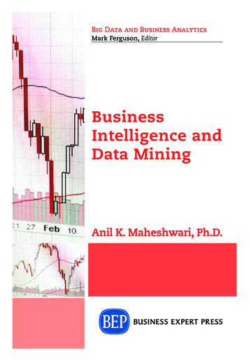
8Data Mining and AnalysisX2(1, 4)bc4a bbc3b21(5, 3)aθX10012345Figure 1.3. Distance and angle. Unit vectors are shown in gray.Because the smallest angle θ [0 , 180 ] and because cos θ [ 1, 1], the cosinesimilarity value ranges from 1, corresponding to an angle of 0 , to 1, correspondingto an angle of 180 (or π radians).OrthogonalityTwo vectors a and b are said to be orthogonal if and only if aT b 0, which in turnimplies that cos θ 0, that is, the angle between them is 90 or π2 radians. In this case,we say that they have no similarity.Example 1.3 (Distance and Angle). Figure 1.3 shows the two vectors 51a and b 34Using Eq. (1.1), the Euclidean distance between them is given asp δ(a, b) (5 1)2 (3 4)2 16 1 17 4.12The distance can also be computed as the magnitude of the vector: 514a b 34 1p because ka bk 42 ( 1)2 17 4.12.The unit vector in the direction of a is given as 11a550.86 ua 0.51kak52 32 334 3

91.3 Data: Algebraic and Geometric ViewThe unit vector in the direction of b can be computed similarly: 0.24ub 0.97These unit vectors are also shown in gray in Figure 1.3.By Eq. (1.3) the cosine of the angle between a and b is given as T 5134117cos θ 222234 175 3 1 42We can get the angle by computing the inverse of the cosine: θ cos 1 1/ 2 45 Let us consider the Lp -norm for a with p 3; we getkak3 53 33 1/3 (153)1/3 5.34The distance between a and b using Eq. (1.2) for the Lp -norm with p 3 is given aska bk3 (4, 1)T3 43 ( 1)3 1/3 (63)1/3 3.981.3.2 Mean and Total VarianceMeanThe mean of the data matrix D is the vector obtained as the average of all thepoints:nmean(D) µ 1Xxin i 1Total VarianceThe total variance of the data matrix D is the average squared distance of each pointfrom the mean:1X1Xkxi µk2δ(xi , µ)2 n i 1n i 1nvar(D) n(1.4)Simplifying Eq. (1.4) we obtainnvar(D) 1Xkxi k2 2xTi µ kµk2n i 1 Xnn11 Xkxi k2 2nµTxi n kµk2 n i 1n i 1!

10Data Mining and Analysisn1 Xkxi k2 2nµT µ n kµk2 n i 1!n1 Xkxi k2 kµk2 n i 1!The total variance is thus the difference between the average of the squared magnitudeof the data points and the squared magnitude of the mean (average of the points).Centered Data MatrixOften we need to center the data matrix by making the mean coincide with the originof the data space. The centered data matrix is obtained by subtracting the mean fromall the points: T T T Tz1x1 µTµx1 T T T TT x2 µ x2 µ z2 Z D 1 · µT . . . . . . . . xTn µTµTxTn(1.5)zTnwhere zi xi µ represents the centered point corresponding to xi , and 1 Rn is then-dimensional vector all of whose elements have value 1. The mean of the centereddata matrix Z is 0 Rd , because we have subtracted the mean µ from all the points xi .1.3.3 Orthogonal ProjectionOften in data mining we need to project a point or vector onto another vector, forexample, to obtain a new point after a change of the basis vectors. Let a, b Rm be twom-dimensional vectors. An orthogonal decomposition of the vector b in the directionX2b43r ab 21p bkX10012345Figure 1.4. Orthogonal projection.

111.3 Data: Algebraic and Geometric Viewof another vector a, illustrated in Figure 1.4, is given as(1.6)b bk b p rwhere p bk is parallel to a, and r b is perpendicular or orthogonal to a. The vectorp is called the orthogonal projection or simply projection of b on the vector a. Notethat the point p Rm is the point closest to b on the line passing through a. Thus, themagnitude of the vector r b p gives the perpendicular distance between b and a,which is often interpreted as the residual or error vector between the points b and p.We can derive an expression for p by noting that p ca for some scalar c, as p isparallel to a. Thus, r b p b ca. Because p and r are orthogonal, we havepT r (ca)T (b ca) caT b c2 aT a 0which implies thataT baT aTherefore, the projection of b on a is given as T a bap bk ca aT ac (1.7)Example 1.4. Restricting the Iris dataset to the first two dimensions, sepal lengthand sepal width, the mean point is given as 5.843mean(D) 3.054X2ℓ1.5rSrSrS1.0rs rsrSrs rsrSrsrSrS0.5rSrSrS0.0rSrSrSrSrSrSrSrSrSrSrSrs rsrSrSrSrSrSuTrS rs rs rs rs rSrs rsrs rsrSrs rsrs rs rsrs rS rsrsbCbCbCbCbCbc tucb bcbCrSuTuTbc ut bc bcuTbCbCbCbCbCbCbc utbc ut CuTbbcut bc bcbCbc ut bcuTbCuTut bcut Cbbc ut bcutbc bcut 2.0uTbCuTbCuTbCuTuTuTuTbCuTbCbcut utbCuTbCbCuTbCuTuTuTbCuTX1uTuTuTbCbCuTuTuTut CuTbbcutbcut bcbC

This book is an outgrowth of data mining courses at Rensselaer Polytechnic Institute (RPI) and Universidade Federal de Minas Gerais (UFMG); the RPI course has been offered every Fall since 1998, whereas the UFMG course has been offered since 2002. Although there are several good boo