Transcription
Graph-Based Deep Modeling and Real Time Forecasting ofSparse Spatio-Temporal DataBao Wang, Xiyang Luo, Fangbo Zhang Baichuan Yuan, Andrea L. BertozziDept of Math, UCLA, Los Angeles, ath.ucla.eduABSTRACTWe present a framework for spatio-temporal (ST) data modeling,analysis, and forecasting, with a focus on data that is sparse in spaceand time. Our multi-scaled framework couples two components: aself-exciting point process that models the macroscale statisticalbehaviors of the ST data and a graph structured recurrent neuralnetwork (GSRNN) to discover the microscale patterns of the STdata on the inferred graph. This novel deep neural network (DNN)incorporates the real time interactions of the graph nodes to enablemore accurate real time forecasting. The effectiveness of our methodis demonstrated on both crime and traffic forecasting.CCS CONCEPTS Information storage and retrieval Time series analysis; Applied computing Social sciences;KEYWORDSSparse Spatio-Temporal Data, Spatio-Temporal Graph, Graph Structured Recurrent Neural Network, Crime Forecasting, Traffic Forecasting.ACM Reference format:Bao Wang, Xiyang Luo, Fangbo Zhang, Baichuan Yuan, Andrea L. Bertozzi,and P. Jeffrey Brantingham. 2018. Graph-Based Deep Modeling and RealTime Forecasting of Sparse Spatio-Temporal Data. In Proceedings of , London,United Kingdom, August 2018 (MiLeTS ’18), 9 pages.DOI: 10.475/123 41INTRODUCTIONAccurate spatio-temporal (ST) data forecasting is one of the centraltasks for artificial intelligence with many practical applications. Forinstance, accurate crime forecasting can be used to prevent criminalbehavior, and forecasting traffic is of great importance for urbantransportation system. Forecasting the ST distribution effectivelyis quite challenging, especially at hourly or even finer temporalscales in micro-geographic regions. The task becomes even harder BaoWang, Xiyang Luo, and Fangbo Zhang contributed equally.Permission to make digital or hard copies of part or all of this work for personal orclassroom use is granted without fee provided that copies are not made or distributedfor profit or commercial advantage and that copies bear this notice and the full citationon the first page. Copyrights for third-party components of this work must be honored.For all other uses, contact the owner/author(s).MiLeTS ’18, London, United Kingdom 2018 Copyright held by the owner/author(s). 123-4567-24-567/08/06. . . 15.00DOI: 10.475/123 4P. Jeffrey BrantinghamDept of Anthropology, UCLA, Los Angeles, CA90095-1555branting@ucla.eduwhen the data is spatially and/or temporally sparse. There are manyrecent efforts devoted to quantitative study of ST data, both fromthe perspective of statistical modeling of macro-scale propertiesand deep learning based approximation of micro-scale phenomena.In [15], Mohler et al. pioneered the use of the Hawkes process (HP)to predict crime, and recent field trials show that it can outperformcrime analysts, and are now used in commercial software deployedin over 50 municipalities worldwide.This paper builds on our previous work [21] in which we appliedST-ResNet, along with data augmentation techniques, to forecastcrime on a small spatial scale in real time. We further showed thatthe ST-ResNet can be quantized for crime forecasting with only anegligible precision reduction [20]. Moreover, ST data forecastingalso has wide applications in computer vision [5–7, 11, 12]. PreviousCNN-based approaches for ST-data forcasting use a rectangular grid,with temporal information represented by a histogram on the grid.Then, a CNN is used to predict the future histogram. This prototypeis sub-optimal from two aspects. First, the geometry of a city isusually highly irregular, resulting in the city’s spatial area takingup a small portion of its bounding box, introducing unnecessaryredundancy in the algorithm. Moreover, the spatial sparsity isexacerbated by the spatial grid structure. Directly applying a CNNto fit the extreme sparse data can lead to all zero weights due tothe weight sharing of CNNs [20]. This can be alleviated by usingspatial super-resolution[20], with increased computational cost.Moreover this lattice based data representation omits geographicalinformation and spatial correlation within the data itself.In this work, we develop a framework to model sparse and unstructured ST data. Compared to previous ad-hoc spatial partitioning, we introduce an ST weighted graph (STWG) to represent thedata, which automatically solves the issue caused by spatial sparsity.This STWG carries the spatial cohesion and temporal evolution ofthe data in different spatial regions over time. Unlike the fast Kronecker approach [17], we infer the STWG by solving a statisticalinference problem. For crime forecasting, we associate each graphnode with a time series of crime intensity in a zip code region,where each zip code is a node of the graph. As is shown in [15], thecrime occurrence can be modeled by a multivariate Hawkes process(MHP), where the self and mutual-exciting rates determines theconnectivity and weights of the STWG. To reduce the complexity ofthe model, we enforce the graph connectivity to be sparse. To thisend, we add an additional L 1 regularizer to the maximal likelihoodfunction of MHP. The inferred STWG incorporates the macroscaleevolution of the crime time series over space and time, and is much
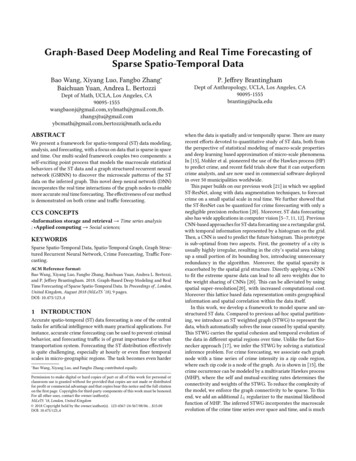
MiLeTS ’18, August 2018, London, United KingdomDataGraphDNNB. Wang et al.OutputFigure 1: Flow chart of the algorithm.more flexible than the lattice representation. To perform microscale forecasting of the ST data, we build a scalable graph structuredRNN (GSRNN) on the inferred graph based on the structural-RNN(SRNN) architecture [7]. Our DNN is built by arranging RNNs in afeed-forward manner: We first assign a cascaded long short-termmemory (LSTM) (we will explain this in the following paragraph)to fit the time series on each node of the graph. Simultaneously,we associate each edge of the graph with a cascaded LSTM thatreceives the output from neighboring nodes along with the weightslearned from the Hawkes process. Then we feed the tensors learnedby these edge LSTMs to their terminal nodes. This arrangement ofedge and node LSTMs gives a native feed-forward structure that isdifferent from the classical multilayer perceptron. A neuron is thebasic building block of the latter, while our GSRNN is built withLSTMs as basic units. The STWG representation together with thefeed-forward arranged LSTMs build the framework for ST dataforecasting. The flowchart of our framework is shown in Fig. 1.Our contribution is summarized as follows: We employ a compact STWG to represent the ST sparseunstructured data, which automatically encodes importantstatistical properties of the data. We propose a simple data augmentation scheme to allowDNN to approximate the temporally sparse data. We generalize the SRNN[7] to be bi-directional, and applya weighted average pooling which is more suitable for STdata forecasting. We achieve remarkable performance on real time crimeand traffic forecasting at a fine-grained scale.In section 2, we briefly review the literature of time-series forcasting. In section 3, we describe the datasets used in this work,including data acquisition, preprocessing, spectral and simple statistical analysis. In section 4, we present the pipeline for generalST data forecasting, which contains STWG inference, DNN approximation of the historical signals, and a data augmentation scheme.Numerical experiments on the crime and traffic forecasting tasksare demonstrated in sections 5 and 6, respectively. The concludingremarks and future directions are discussed in section 7.2RELATED WORKA lot of study have utilized deep learning to study the forecasting ofST time series, most of which involves a CNN structure to capturethe spatial information, and a RNN structure to model temporaldependency. In [8], the authors implemented CNN to extract thefeatures from the historical crime data, and then used a supportvector machine (SVM) to classify whether there will be crime ornot at the next time slot. Zhang et al.[22] create an ensemble ofresidual networks [4], named ST-ResNet, to study and predict trafficflow. Graph-based diffusion on RNN [14] is also proposed for trafficforecasting. Additional applications include [7] who use the STgraph to represent human environment interaction, and proposeda structured RNN for semantic analysis and motion reasoning. Thecombination of video frame-wise forecasting and optical flow interpolation allows for the forecasting of the dynamical process ofthe robotics motion [6]. RNNs have also been combined with pointprocesses to study taxi and other data [2]. The closest to this workis by Wang et al.[21], who used ST-ResNet to forecast crime on asmall spatial scale in real time.3DATASET DESCRIPTION AND SIMPLEANALYSISWe study two different datasets: the crime and traffic data. Theformer is more irregular in space and time, and hence is much morechallenging to study. In this section we describe these datasets andintroduce some preliminary analyses.3.1Crime Dataset3.1.1 Data Collection and Preprocessing. We consider crime datain Chicago (CHI) and Los Angeles (LA). In our framework, historicalcrime and weather data are the key ingredients. Holiday information, which is easy to obtain, is also included. The time intervalsstudied are 1/1/2015-12/31/2015 for CHI and 1/1/2014-12/31/2015for LA, with a time resolution of one hour. Here we provide a briefdescription of the acquisition of these two critical datasets.Weather Data. We collect the weather data from the WeatherUnderground data base1 through a simple web crawler. We select temperature, wind speed, and special events, including fog,snow, rain, thunderstorm for our weather features. All data isco-registered in time to the hour.Crime Data. The CHI crime data is downloaded from the Cityof Chicago open data portal. The LA data is provided by the LAPolice Department (LAPD). Compared to CHI data, the LA crimedata is sparser and more irregular in space. We first map the crimedata to the corresponding postal code using QGIS software [18].A few crimes in CHI (less than 0.02%) cannot be mapped to thecorrect postal code region, and we simply discard these events. Forthe sake of simplicity, we only consider zip code regions with morethan 1000 crime events over the full time period. This filteringcriterion retains over 95 percent of crimes for both cities, leavingus with 96 postal code regions in LA and 50 regions in CHI.3.1.2 Spectrum of the Crime Time Series. Figure 2 plots thehourly crime intensities over the entire CHI and a randomly selectedzip code region. Though the time series are quite noisy, the spectrumexhibits clear diurnal periodicity with magnitude peaked at 24hours, as shown in Fig. 3.3.1.3 Statistical Analysis of Crime Data. Evidence suggests thatcrime is self-exciting [16], which is reflected in the fact that crimeevents are clustered in time. The arrival of crimes can be modeledas a Hawkes process (HP) [15] with a general form of conditionalintensity function:Õλ(t) µ aд(t ti )(1)t i twhere λ(t) is the intensity of events arrival at time t, µ is the endogenous or background intensity, which is simply modeled by1 https://www.wunderground.com/
Graph-Based Deep Modeling and Real Time Forecasting of Sparse Spatio-Temporal DataMiLeTS ’18, August 2018, London, United Kingdom(a) ExactFigure 2: Example plots of the hourly crime intensities forthe entire 2015 CHI (left) and the 2015 60620 zip code (right).(b) one path sampled(c) ensemble 5000Figure 4: Exact and simulated hourly crime intensities forCHI 60620 in the first two weeks of Nov 2015. (a), (b), and(c) depict the exact, one path sampled from the HP, and theensemble average of 5000 paths, respectively.3.2Traffic DataWe also study the ST distribution of traffic data [22]. The datacontains two parts: taxi records from Beijing (TaxiBJ) and bicycledata from New York city (BikeNYC). Basic analyse in [22] showsperiodicity, meteorological dependence, and other basic propertiesof these two datasets. The time span for TaxiBJ and BikeNYC areselected time slots from 7/1/2013 to 4/10/2016 and the entire span4/1/2014-9/30/2014, respectively. The time intervals are 30 minutesand one hour, respectively. Both data are represented in Eulerianrepresentations with lattice sizes to be 32 32 and 16 8, respectively.Traffic flow prediction using this traffic dataset will be selected asbenchmark to evaluate our model.4Figure 3: Spectrum of the time series from Fig. 2. (log-scalein y-axis.)a constant, a is the self-exciting rate, and д(t) is a kernel triggering function. In [24], it found that an exponential kernel, i.e.,д(t) w exp( wt) where w1 models the average duration of theinfluence of an event, is a good description of crime self-excitation.To calibrate the HP, we use the expectation-maximisation (EM)algorithm [19]. Simulation of the HP is done via a simple thinningalgorithm [10].The HP fits to the crime time series in zip code region 60620 yieldsÍλ(t) 0.7562 ti t 0.4673 31.6301 exp( 31.6301 (t ti )), whichshows that on average, each crime will have 0.4673 offspring. Furthermore, we noticed that the duration of the influence is roughlya constant over different zip code regions.Figure 4 shows the exact and simulated crime intensities in thefirst two weeks in Nov 2015 over zip code region 60620. Both the exact and simulated time series demonstrate clustered behavior, whichconfirms the assumption that crime time series is self-exciting, andsupports the contention that the HP is a suitable model. However,the simulate intensity peaks are shifted relative to the exact ones.If we use the HP to do the crime forecasting, we typically do anensemble average of many independent realizations of the HP, as isshown in panel (c). However, this ensemble average differs hugelyfrom the exact crime time series. To capture fine scale patterns wewill use DNN.ALGORITHMS AND MODELSOur model contains two components. The first part is a graph representation for the ST evolution of the data, where the nodes of thegraph are selected to contain sufficient predictable signals, and thetopological structure of the graph is inferred from self-exciting pointprocess model. The second component is a DNN to approximatethe temporal evolution of the data, which has good generalizability.The advantages of a graph representation are two-fold: on the onehand, it captures the irregularity of the spatial domain; on the otherhand, it can capture versatile spatial partitioning which enablesforecasting at different spatial scales. In this section, we will presentthe algorithms for modeling and forecasting the ST sparse unstructured data. The overall pipeline includes: STWG inference, dataaugmentation, and the structure and algorithm to train the DNN.4.1STWG Representation for the ST DataThe entire city is partitioned into small pieces with each piece representing one zip code region, or other small region. This partitioningretains geographical cohesion. In the STWG, we associate eachgeographic region with one node of the graph. The inference ofthe graph topological structure is done by solving the maximallikelihood problem of the MHP. We model the time series on thegraph by the following MHP {Ntu u 1, 2, · · · , U } with conditionalintensity functions:Õλu (t) µu auui д(t ti ),(2)i:t i twhere µu 0 is the background intensity of the process for theu-th node and ti is the time at which the event occurred on node uiprior to time t. The kernel is exponential, i.e., д(t) w exp( w t).
MiLeTS ’18, August 2018, London, United KingdomB. Wang et al.We calibrate the model in Eq.(2) using historical data. Let µ (µu u 1, 2, · · · , U ) and A (auu 0 u, u 0 1, 2, · · · , U ). Supposewe have m i.i.d samples {c 1 , c 2 , · · · , cm } from the MHP; each isa sequence of events observed during a time period [0,Tc ]. Theevents form a set of pairs (tic , uic ) denoting the time tic and the nodeuic -th for each event. The log-likelihood of the model is:!ncU TcÕÕ ÕcL(µ, A) log λui (ti ) λu (t)dt .(3)ci 1u 1 0Similar to the work by Zhou et al. [23], to ensure the graph isÍsparsely connected, we add an L 1 penalty, λ A 1 λ uu 0 auu 0 , tothe log-likelihood L in Eq.(3): Lλ (µ, A) L λ A 1 . To infer thegraph structure, we solve the optimization problem:argmin µ,A Lλ (µ, A),Figure 5: Plot of w vs log-likelihood. The maximum valueoccurs at w 20 and w 18 respectively for CHI and LA.s.t. µ 0, and A 0,where µ 0 and A 0, both are defined element-wise. We solvethe above constraint optimization problem by the EM algorithm.The L 1 constraint is solved by a split-Bregman liked algorithm [3].For a fixed parameter w, we iterate between the following two stepsuntil convergence is reached: E-Step: Compute the exogenous or endogenous probability:(k )cpii µu c(a) CHIi(k )µu c iÍi 1 (k )ccj 1 au i u j д(ti t j )(b) LA,aui u j д(tic t jc )(k ) Í(k )ccµu c i 1j 1 au i u j д(ti t j )Figure 6: Image plot of the self and mutual excitation matrixA for the cities CHI and LA.(k )picj i M-Step: Update parameters:(k 1)µu(k 1)auu 0nc1 Õ Õcªpii c Tccci 1,u u« i Í1/2Í(k ) Í Íc auu 0 c i:uic u j i,u jc u 0 pi j ª Tc t jcÍ Íc u 0д(t)dtcj:u0j« (k 1)(k 1)auu 0 shrinkλ (auu 0 ).The above EM algorithm is of quadratic scaling, which is infeasiblefor our datasets. To reduce the algorithm’s complexity, insteadof considering all events before a given time slot, we do a simpletruncation in the E-step based on the localization of the exponentialkernel. This truncation simplifies the algorithm from quadraticscaling to almost linear scaling. In the inference of the STWG, weset the hyper-parameter λ to be 0.01.4.1.1 Results on STWG Inference. Due to the high conditionnumber of the log-likelihood function with respect to the parameterw [24], we perform a simple grid search to find the optimal w (seeFig. 5). The likelihood functions are maximized when w is 20 and18 for CHI and LA, respectively. The similarity between the optimalduration parameters for Chicago and Los Angeles suggest that theduration of the self-excitation is an intrinsic property of crime. Theoptimal self-excitation parameters sets A for two cities are plotted inFig.6. The diagonal in Fig. 6 reflects the intensity of self-excitationwithin a single node of the graph (i.e., zip code region). Off-diagonalentries reflects self-excitation of crime between nodes of the graph.Only nodes that demonstrate self-excitation above a threshold thetaare connected by an edge in the final graph.4.1.2 Effectiveness of STWG Inference. We validate the efficacyof the inference algorithm on a synthetic problem. To generate thesynthetic data, a random graph G is first generated with a fixed levelof sparsity on a fixed set of nodes i 1, . . . , U . A MHP E is thensimulated for a fixed amount of time T with randomly generatedbackground rate µ i , and excitation rates ai, j supported on the graphG. We use the aforementioned algorithm to infer the coefficientsâi, j . To obtain the underlying graph structure, there is an edgeconnected from node j to i if and only if Sign(âi, j θ ) 0, where θis a threshold that determines the sparsity of the inferred weightedgraph. To evaluate the efficacy of the inference algorithm, we varythe threshold θ to obtain a ROC curve, where a connection betweentwo nodes i and j is treated as positive and vice versa. The areaunder the ROC curve (AUC) will be a metric on the performance ofthe algorithm.For the experiments, we generate a directed and fully connectedgraph G with N 30 nodes, and keep each edge ei j with probability s 0.1, 0.2, . . . , 0.5, where s denotes the sparsity levelof the graph. We generate at random µ i U ni f ([0, 0.1]) andai, j U ni f ([0.02, 0.1]) for i, j connected in G, and 0 otherwise.And we check the stability condition in the spectral norm whereρ(A) 1. A HP is then simulated with T 3 104 . In crime networks, it is reasonable to assume that the interactions ai j are local,and hence we may start out with a reduced set of edges during the
Graph-Based Deep Modeling and Real Time Forecasting of Sparse Spatio-Temporal DataMiLeTS ’18, August 2018, London, United KingdomTable 1: AUC of the ROC curve for the graph inference problem. Rows denote the sparsity of the ground truth graph,columns are different prior knowledge for network structure for the inference 8970.8840.9150.910GT 2000.9890.9870.9820.9810.986GT igure 8: The architecture of the cascaded LSTM that usedfor single node data modeling.Figure 9: Histogram of the hourly crime counts in zip coderegions 60620, for the year 2015, and 90003, for 2014-2015.(a) GT(b) GT 200(c) GT 400Figure 7: Visualization of the ground truth and inferredgraph for the synthetic data. The inferred graphs were obtained by thresholding ai j to match the sparsity level of theoriginal network. The true positives, true negatives, falsepositives, false negatives are color coded in yellow, blue, red,green respectively.inference procedure to increase accuracy of the network recovery.Therefore, in addition to recovering the network structure from afully connected graph, we also test the inference algorithm on aset of reduced edges that contain the ground truth. For simplicity,we randomly choose 200 and 400 edges from the graph and addthem to the true network structure at initialization. We observethat the inference algorithm is able to obtain an AUC of around 0.9across all levels of sparsity, with large increases in performance ifthe graph prior is narrower.4.2Data Augmentation - Single Node StudyWe consider data augmentation to boost the performance of theDNN for sparse data forecasting, with single zip code crime forecasting as an illustration. In our previous work [20, 21], when dealingwith crime forecasting on a square grid, we noticed the DNN poorlyapproximates the crime intensity function. However, it does approximate well the diurnal cumulated crime intensity, which hasbetter regularity. According to the universal approximation theorem [1], the DNN can approximate any continuous function witharbitrary accuracy. However, the crime intensity time series is farfrom a continuous function due to its spatial and temporal sparsityand stochasticity. Mathematically, consider the diurnal time series {x(t)} with period T . We map {x(t)} to its diurnal cumulativefunction via the following periodic mapping: ty(t) x(s)ds I (x(t)),(4)nTfor t [nT , (n 1)T ), this map is one-to-one.We also super-resolve the diurnal cumulated time series {y(t)} toconstract an augmented time series {ŷ(T )} on half-hour incrementsvia linear interpolation. The new time series has a period of T̂ 2T 1. In the time interval [nT̂ , (n 1)T̂ ) it is defined as:(y(nT k)t nT̂ 2kŷ(t) 1(5)[y(nT k) y(nT k 1)]t nT̂ 2k 1,2for k 0, 1, · · · ,T 1. It is worth noting the above linear interpolation is completely local. In the following DNN training procedureit will not lead to information leak.4.2.1 Cascaded LSTM for Single Node Crime Modeling. The architecture of the DNN used to model single node crime is a simplecascaded LSTM as depicted in Fig.8. The architecture contains twoLSTM layers and one fully-connected (FC) layer, and represents thefollowing function:DNN(x) FC LSTM1 LSTM2 (x),(6)where x is the input. Generally, we can cascade N layers of LSTM.In the above cascaded architecture, all the LSTMs are equippedwith 128 dimensional outputs except the first one with 64 dimensions. An FC layer maps the input tensor to the target value. Toavoid information leak when applying DNN to the super-resolvedtime series, we skip the value at the nearest previous time slot inboth training and generalization.Before fitting the historical crime intensities by the cascadedLSTMs, we first look at histograms of the crime intensities (Fig.9).The 99th percentiles of crime distributions are each less than sixcrimes. This suggests that local crime intensity is important andone cannot use a simple binary classifier.We adopt the two layers of LSTMs cascade, which is demonstrated in Fig.8 to fit the single node crime time series. To trainthe DNNs for a single node, we run 200 epochs with the ADAMoptimizer [9], starting from the initial learning rate 0.01 with decayrate 1e 6. Fig. 10 shows the decay of the loss function for the rawcrime time series and cumulated super-resolved (CS) time series inpanels (a) and (b), respectively. It can be seen from the figure that
MiLeTS ’18, August 2018, London, United KingdomB. Wang et al.NLosstrainingvalidation0.02raw data0.010050augmented data100150Epochs200Figure 10: Training procedures of the different scenarios onthe node 90003. Evolution of the training and validation losson the raw data and on the augmented data.DNN performs much better on the regularized time series than theraw one, i.e. the loss function reaches a much lower equilibrium.To show the advantage of the generalization ability of the DNN,we compare it with a few other approaches, including autoregressive integrated moving average (ARIMA), K-nearest neighbors(KNN), and historical average (HA). For sparse data, we fit thehistorical data and perform one step forecasting in the same manner as our previous work [20]. The root mean squared error (RMSE)between the exact and predicted crime intensities and optimal parameters for the corresponding model are listed in Table 2. Underthe RMSE measure, DNN, especially on the augmented data, yieldshigher accuracy. The small RMSE reflects the fact that DNN approximates the crime time series with good generalization ability.Table 2: RMSE between the exact and predicted crime intensities over the last two months of 2015, in the region withzip code 90003. DNN(CS) denotes DNN model applied to theaugmented data. Comparison with more advanced baselinemodels will be given in the rest of this paper.MethodsRMSE (number of crimes)DNN0.858DNN (CS)0.491ARIMA(25, 0, 26)0.941KNN (k 1)1.193HA0.904However, the simple RMSE measure is insufficient to measureerror appropriately for sparse data. Do HA and ARIMA really workbetter than KNN for crime forecasting? HA ignores the day to dayvariation, while ARIMA simply predicts the number of crimes tobe all zeros after flooring. KNN predicts more useful informationthan both ARIMA and HA for the crime time series. We proposethe following measure, which we call a “precision matrix” (do notconfuse it with the one used in statistics) B be defined as:β 10 . B .« βm0···.···β 1n.βmnª where βi j Niij , where Ni #{t x t i}, and Ni j #{t x t pppi and (x t i or x t 1 i or · · · or x t j 1 i)}, for i 1, 2, · · · n;pj 0, 1, · · · , m. Here x t and x t are the exact and predicted numberof crimes at time t. This means for a given threshold number ofcrimes i, we count the number of time intervals in the testing set atwhich the predicted and exact number of crimes both exceed thisthreshold i, with an allowable delay j, i.e., the prediction is allowedwithin j hours earlier than the exact time.This measure provides much better guidance for crime patrolstrategies. For instance, if we forecast more crime to occur in agiven patrol area, then we can assign more police resources to thatarea. This metric allows for a few hours of delay but penalizesagainst crimes happening earlier than predicted, due to the timeirreversibility of forecasting. For the crime time series in nodes60620 and 90003, we select m 3, n 2 and m 5, n 4,respectively, based on the sparsity level. Fig. 11 shows the precisionmatrices of the crime prediction by different methods, confirmingthat DNN together with data augmentation gives accurate crimeforecasting. Meanwhile, the KNN also gives better results comparedto other methods except the DNN with data augmentation. Thiscorrects potential inaccuracies in the RMSE measure and confirmsthe spatial correlation of the crime time series.Remark 1. The precision matrix B still has an issue in the case ofover-prediction. Namely, this measure fails to penalize cases wherethe prediction is higher than the ground truth. However in those cases,the RMSE would typically be very large. Therefore, to determine if thesparse data is well predicted or not, we should examine both metrics.Another merit of the DNN is that with sufficient training data,as the network goes deeper, better generalization accuracy can beachieved. To validate this, we test the 2 and 3 layers LSTM cascadeson the node 60620 (see Fig. 12).4.3GSRNN for ST ForecastingOur implementation of the GSRNN is based on the SRNN implementation in [7] (Fig.13), but differs in these key aspects: 1) Wegeneralize the SRNN model to a directed graph, which is moresuited to the ST data forecasting problem. 2) We use a weightedsum pooling based on the self-exciting weights from the MHP inference. 3) Due to the large number of nodes in the graph, wesubsample each class of nodes for scalability.To be more specific, suppose i 1, 2, . . . N are the nodes ofthe graph, and X i (t) denotes value of the time series at time t fornode i. We first deploy the STWG inference procedure to obtain theweighted directed graph, with weight on the edge connecting node iand j denoted as w i j . With the same setup as in [7], we partition thegraph nodes to K groups according to some criterion. We construct2 for eachan “input RNN” Ek1 for each class k, and an “edge RNN” Ek,lclass pair (k, l) if k , l. For the forward pass, if node i belongs toclass k, we feed a set of historical data {X i (t p) p n 1 , n 2 , ., nm }2 . Into Ek1 , and the data from neighboring nodes of class l to Ek,lcontrast to [7], we use a weighted sum
correct postal code region, and we simply discard these events. For the sake of simplicity, we only consider zip code regions with more than 1000 crime events over the full time period. „is ltering criterion retains over 95 percent of crimes for both cities, leaving us with 96 postal