Transcription
M. E. Adeosun, S. O. Edeki, O. O. UgbeborWSEAS TRANSACTIONS on MATHEMATICSStochastic Analysis of Stock Market Price Models: A Case Study ofthe Nigerian Stock Exchange (NSE)M. E. ADEOSUNS. O. EDEKIOsun State College of TechnologyCovenant UniversityDepartment of Mathematics & Statistics Department of Mathematical SciencesEsa-OkeCST, oo.comO. O. UGBEBORUniversity of IbadanDepartment of : In this paper, stochastic analysis of the behaviour of stock prices is considered using a proposed lognormal distribution model. To test this model, stock prices for a period of 19 years were taken from the NigerianStock Exchange (NSE) for simulation, and the results reveal that the proposed model is efficient for the predictionof stock prices. Better accuracy of results via this model can be improved upon when the drift and the volatilityparameters are structured as stochastic functions of time instead of constants parameters.Key–Words: Stochastic model, lognormal distribution, random walk, option pricing, stock exchange market1Introductionwith positive probability, and ignores the discountingwhich in reality is not visible, this model was refinedby Osborne model in [3], who stated that the log returnof the stock process should follow a normal distribution with mean zero and variance σ 2 τ for any smallτ 0. Shortly, the geometric Brownian Motion wasintroduced in [4], where the price of the risky stockevolves according to the SDE:The stock price is one of the highly volatile variablesin a stock exchange market. The unstable propertyand other considerable factors such as liquidity on stock return [1] call for concern on the part of investors,since the sudden change in share prices occurs randomly and frequently. Researchers are therefore propelled to look into the behavior of the unstable marketvariable so as to advise investors and owners of cooperation who are looking for convenient ways to raisemoney by issuing shares of stocks in their cooperation.The basis of this work lies in the observation ofthe Scottish botanist Robert Brown in [2]. This is sosince the path of the stock price process can be linkedto his description of the random collision of some tinyparticles with the molecules of the liquid, he introduced what is called Brownian motion. The “Arithmetic” Brownian motion in the Bachelier’s model wasthe first mathematical model of stock [2]. The stockprice model proposed by Bachelier assumed that thediscount rate is zero while the dynamics of the stocksatisfies the following stochastic differential equation(SDE):dS(t) S0 σdW (t)(1)dS(t) µS(t)dt σS(t)dW (t)where µ is the expected rate of share price changes ina given trading period, while other parameters are asearlier defined.In (2), there is an assumption that the option derived from a stock has a constant expected rate of return µ. In [5, 6], Black and Schole contributed to theworld of finance via the introduction of Ito calculusto financial mathematics, and also the Black-Scholesformula. Brennan and Schwarz in [7] employed a finite difference method for pricing the American option for the Black-Schole model. This led to the onedimensional parabolic partial differential inequality.The main shortcoming of the Black-Schole model is its constant volatility assumption. Meanwhile,statistical analysis of the stock market data shows thatthe volatility of the stock is a time dependent quantity,and also exhibits various random features. Stochasticvolatility of models like the Hull-white model in [8]addressed the randomness by assuming that both thestock price and the volatility are stochastic processesaffected by the different sources of risk.The equation in a stochastic model for stock pricewhere S(t) is the spot price of the underlying assets attime t, W (t) a standard Brownian motion, and σ thevolatility of the stock price.As a result of the shortcoming of Bachelier’smodel which states that the hypothesis of the absoluteBrownian motion in (1) leads to a negative stock price1E-ISSN: 2224-2880(2)353Volume 14, 2015
M. E. Adeosun, S. O. Edeki, O. O. UgbeborWSEAS TRANSACTIONS on MATHEMATICSvolatility in financial engineering was combined withthe concept of potential energy in econophysics [9].In the improved equation, random walk term in thestochastic model was multiplied by the absolute value of the difference between the current price and theprice in the previous period divided by the square rootof a time step raised to the power of a certain value,and then added to a term which is the price differencemultiplied by a coefficient.McNicholas and Rzzo [10] applied the Geometric Brownian Motion (GBM) model to simulate futuremarket prices. Also, the Cox-ingersoll-Ross approachwas used by them to derive the integral interest generator and through stochastic simulation, the result wasa full array of price outcomes along with their respective probabilities. The model was used to forecast stock prices of the sampled banks in the five weeks in1999. Since, the stock prices fluctuate as quickly aspossible, a determination of an equilibrium price anda dynamic stability is somewhat tasking. Osu [11] determined the equilibrium price of a solution of the stock pricing PDE which is the backward Black-ScholePDE in one variable. This was with regard to different values of the interest rate. For stochastic nature offinancial model; Edeki et al [12] considered the effectof stochastic capital reserve on actuarial risk analysis.Ugbebor et al [13] considered an empirical stochasticmodel of stock price changes. Fama [14, 15] presented random walks and stock behavior with respect tostock market prices.In modeling stock prices, Dmouj [16], constructed the GBM and studied the accuracy of the modelwith detailed analysis of simulated data. ExponentialLevy model for application in finance was consideredin [17]. On the aspect of parameter estimation andmodel prediction in stock prices, much work has beendone, Sorin [18]. In a similar manner, other aspects ofapplied and managerial sciences have been attractingthe attention of researchers with regard to predictivemodels [19, 20].The structure of the remaining part of the paperis as follows: section 2 is on the mathematical formulation of the problem, stock price expected valueand model simulation, and parameters estimation - thevolatility and the drift; section 3 is on data analysisand application of results; while section 4 deals withdiscussion of results and concluding remarks.2The dynamics of the stock price is:dSt µSt dt σSt dWtwhere µSt dt and σSt dWt are the predictable and theunpredictable parts (respectively) of the stock return.Theorem 1 Ito formula Let (Ω, β, µ, F (β)) be a filtered probability space, X {Xi , t 0} be an adaptive stochastic process on (Ω, β, µ, F (β)) possessinga quadratic variation ⟨X⟩ with an SDE defined as:dX(t) g(t, X(t))dt f (t, X(t))dW (t), (4) t IR , and for u u(t, X(t)) C 1 2 ( IR).Then][ u g u 1 2 2 u fdτdu(t, X(t)) t x2 x2 u(5) f dW (t) xEquation (5) whose proof can be found in [6] isa stochastic differential equation (SDE) that can besolved by semi-analytical methods [21, 22] when converted to non SDE of differential type (ODE or PDE).Thus, since the price S(t) of a risky asset such as stockevolves according to the SDE in (4), where W (t) isa standard Brownian motion on the probability space(Ω, β, µ), β σ is the algebra generated by W (t),t 0, µ 0 the drift, and σ the volatility of thestock.Applying Theorem 1 to (3) solves the SDE withthe solution as:S(t) S0 e(µ σ2)t σW (t)2(6)According to the properties of standard Brownian motion process for n 1 and any sequence of time0 t0 t1 · · · tn , therefore by Euler’s methodof discretization of the SDE, we have:ln St ln St 1 (µ σ2) t σ(Wt Wt 1 ) (7)2Remark 2 The random variables W1 Wt 1 are independent and have the standard normal distributionwith mean zero and variance one. Thus, for:Mathematical Formulationy ln St ln St 1 , ξ Wt Wt 1 and t 1.Let S(t) be the stock price of some assets at a specified time t, and µ, an expected rate of returns on thestock, and dt as the return or relative change in theprice during the period of time.Eq. (7) becomes:1yt µ σ 2 σξt22E-ISSN: 2224-2880(3)354Volume 14, 2015(8)
M. E. Adeosun, S. O. Edeki, O. O. UgbeborWSEAS TRANSACTIONS on MATHEMATICS2.2 The Expected value of the stockIn this work, we shall estimate the drift µ, and thevolatility σ, in the next section.Combining (7) and (8) yields:ln St ln St 1 (µ σ2) t σξ( dt)2After determining the volatility (σ) and the drift (µ)of the stock price of the company, the expected stockprice E(St ) is thus defined and denoted as:(())σ22E(St ) exp ln S0 µ t σ t2 )(σ2t exp(ln S0 ) exp µ 2(9)Eq. (9) has the solution given by:St St 1 e(µ σ2) t σξ(2dt)()σ2E(St ) S0 exp µ t.2Eq (15) holds since,() σ2ln St N (ln S0 µ t, σ t).2So(10)Equation (10) shall be used in this work to develop thesimulation of 100 random paths for the stock price foreach respective year using the volatility and the drifteach stock year.Eq. (10) is thus referred to as the geometric Brownian motion model (GBMM) of the future stock priceSt from the initial value S0 . Thus, for the time periodt, when dt t, (10) will therefore become:St S0 e2.1 2(µ σ2 )t σξ( t)Definition 3 The Random walk process. For an integer n, n 0 we define the Random Walk process atthe time t, {Wn (t), t 0} as follows:i. The initial value of the process is:Wn (0) 0(11)ii. The layer spacing between two successive jumpsis equal to n1 ;Stock price expected value and simulation modeliii. The “Up” and “down” jumps are equal and of1size, with equal probability.nLet St denote the (random) price of the stock at timet 0. Then St has a normal distribution if y ln Stis normally distributed.Suppose that y N (µ, σ 2 ), then the pdf of y isgiven as,f (y) 12πσ 2e 12The value of the random walk at the i-th step is defined recursively as follows:( ) ()ii 1XiWn , i 1(16)nnn2( y µσ ) , y ( , ),µ ( , ), σ 0For given constants µ and σ the process has the following form:Bt µt σWt(17)where t represents time and Wt is a random walk process as described in (17), it can also be expressed as: Wt ε t(18)(12)We obtain the lognormal probability density function (pdf) of the stock price St considering the factthat for equal probabilities under the normal and lognormal pdfs, their respective increment areas shouldbe equal.f (y)dy g(St )dStf (y)dy g(St ) dStSubstituting y ln St & dy the pdf of St :g(St ) 11 e2St σ 2πwhere ξ is a random number drawn from a standardnormal distribution.2.3 Parameter Estimation (volatility σ anddrift µ)(13)In the course of developing the random walk algorithm, two parameters have to be estimated; the volatility(σ) and the drift (µ) of the stock price for the selectedcompany. Also, for the purpose of the research, theunit of time is chosen to be one day with which bothparameters will be calculated. The formulae for thevolatility and the drift of the stock price are explainedas follows.dStin (13) definesSt(ln St µσ)2(14)3E-ISSN: 2224-2880(15)355Volume 14, 2015
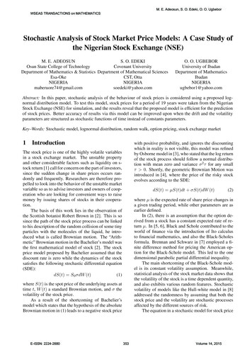
M. E. Adeosun, S. O. Edeki, O. O. UgbeborWSEAS TRANSACTIONS on MATHEMATICSTable 1. Stock Price list from April 1996 till May20142.3.1 The Volatility, σLet Si be the stock price at the end of i-th trading period, τ t, ti 1 , i 1, the length of time intervalbetween two consecutive trading periods, µi the logarithm of the daily return on the stock over the shorttime interval, τ such that:)(Si(19)µi lnSi 1Then the following are defined:1 uinnū (20)i 1vuuν t1 (ui ū)2n 1n(21)i 1νσ .1733.833.41Date(22)where ū is the unbiased estimator of the log return,ui , ν is the standard deviation of the ui ’s and σ thevolatility of the daily stock return.Stock Price2.3.2 The Drift parameter, µThe drift on the other hand is the expected annual rateof return and is determined from the value of the unbiased estimator as follows.()1 2ū 1ū µ σ τ µ σ 2(23)2τ23used in developing the model for the stock price between the years 1997 to the remaining 196 days in2014 using the volatility and the stock of the previousyear from 1996 to 2014 respectively.Using the values of the volatility and the drift ofthe stock price of the year 1996; the value of the stock price for the year 1997 will be determined, withthat of 1997 used to determine the stock price for theyear 1998 etc. Finally, the value of the volatility andthe drift for the year 2014 will be used to predict thevalue of the stock for the remaining days in 2014. Allsimulations in the work are done using MATLAB.Data Analysis and ResultThe data used for the purpose of this research wasfrom a company listed under the Nigerian Stock Exchange (NSE); available on a web platform [23].These consist of historical stock data of 4555 closing stock prices from April 12, 1996 to May 16, 2014.The whole data was subdivided into nineteen smallerdata samples - each sample containing stock price data for a year each with an average of 240 stock tradingdays with a minimum and maximum of 96 and 252days respectively.It is observed from Table 1 that the trading daysfor the year 1996 is 183; that of 1997, and 2008 is 253;that of 1998, 1999, 2000, 2002, 2003, 2004, 2005,2009, 2010, 2011 and 2013 is 252; that of 2001 is248 and that of 2014 is 96. The trading days can beobserved on the first column of Table 1.For the purpose of this study, the generalized random walk (Brownian motion with drift) model was3.1 Analysis and Result of ParametersThe volatility and drift were calculated for each yearusing the stock returns over a period of one year each(see Table 2). Although, the unit period time has anaverage of 240 days per stock year-each respectiveyear was allocated its own unit period given the number of days stated for the stock year; for example a1stock year of 252 days will have a period, τ 252years. Hence, the values of the volatility and drift ofeach respective year was determined.4E-ISSN: 2224-2880356Volume 14, 2015
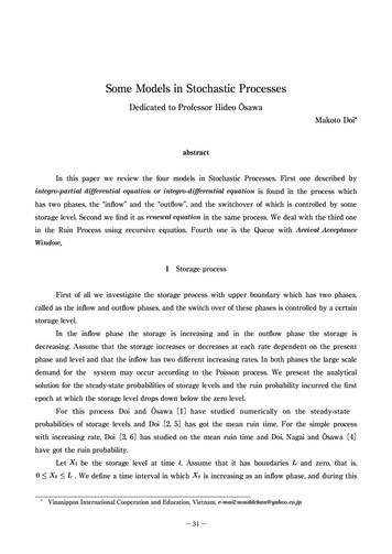
M. E. Adeosun, S. O. Edeki, O. O. UgbeborWSEAS TRANSACTIONS on MATHEMATICSFigure 1: Stock price distributions for the year 1996Figure 3: 100-step random walk and its mean (startingfrom zero)Figure 2: Stock price distributions for the year 1997Figure 4: 1000-step random walk in [0, 1] and itsmean3.1.1 Results of volatility, σ1996, 2006, 2008 and 2014 with a value of -49%, 39%, -38% and -14.6% respectively. The remainingyears have drifts falling within the range of 2% and4%.The distribution of the remaining parameterswhich were also used in determining the drift and thevolatility of the stock is shown in Fig 7 for the estimator of standard deviation/volatility, v and Fig 8 for theunbiased estimator, µ̄.According to Table 2; the distribution of the dailyvolatility of each stock is stated in the 7th column forthe years 1996 till 2014. The highest volatility wasobserved for the year 1998 with a value of 66% whileother years range between 0.2% for 2013, 2% for theyears 2005, 2007, 2010, 2011 and 2014, 3% for theyears 2003, 2006 and 2009, 4% for the year 1996; 5%for the years 2002 and 2008; 6% for the years 1997and 2001 and 7% for the years 1998 and 1999 (seeFig 7 for the plot of the volatility).3.1.23.1.3 Results and discussion of the simulation ofthe stock price for the periodResults of the drift, µFor the simulation of the stock price of the year 1997;the drift and volatility of the year 1996 (see Fig 1 forthe stock price of 1996) which had a value of -0.4908and 0.593452 respectively were used in developingthe simulation of the 100 random walks for the year1996 (see Fig 2). Majority of the simulated plots canbe observed to produce lower stock prices comparedto the actual stock price which shows an increased stock distribution towards the end of the year.For the simulation of the stock price of the year1998; the drift and volatility of the year 1997 whichAccording to the data shown in Table 2, the distribution of the daily drift for the stock price stated for theperiod of 1996 till 2014 is stated in 3rd column. Thedrift which is defined as the daily expected rate of return of the stock for each year shows a varying distribution of the return rate. The highest drift was observed for the years 2013, 1998, 1999 and 2003 witha value of 70%, 184%, 123% and 102% respectively(see Fig 6).The lowest drifts were also recorded for the year2000 with a value of -212% followed by the years5E-ISSN: 2224-2880357Volume 14, 2015
M. E. Adeosun, S. O. Edeki, O. O. UgbeborWSEAS TRANSACTIONS on MATHEMATICSTable 2: Values of the drift, volatility, standard deviation and unbiased estimator for each stock 6Stock 14594705Estimator 7892240.023333683Time intervalτ ty .00182496Figure 7: Volatility/standard deviation, σ of the stockprice for the year 1996 to 2014Figure 5: Estimator of the standard deviation, ν of thestock price for the year 1996 to 2014Figure 8: Unbiased estimator, ū of the stock price forthe year 1996 to 2014Figure 6: Drift, µ of the stock price for the year 1996to 20146E-ISSN: 2224-2880358Volume 14, 2015
M. E. Adeosun, S. O. Edeki, O. O. UgbeborWSEAS TRANSACTIONS on MATHEMATICShas a value of 1.7862 and 0.906322 respectively wereused in developing the simulation of the 100 randomwalks for the year 1998 (see Fig 9) using the initialstock price of 66.25. This can be observed to be asa result of the high volatility of 1998 with a value of10.615442 the year with the highest volatility compared to a volatility of 0.906322 for the year 1997.For the simulation of the stock price of the year1999; the drift and volatility of the year 1998 whichhas a value of 1.8429 and 10.615442 respectively wereused in developing the simulation of the 100 randomwalks for the year 1999 (see Fig 10) using the initial stock price of 24.80. The simulation of the stockprice for the year were out of place due to the difference in the volatility of the stock year with a value of10.615442 for the previous year (1998) while that of1999 is 1.162434. The simulation of the stock pricefor the year 1999 was not a good interpretation of theactual stock price for the year.For the simulation of the stock price of the year2000; the drift and volatility of the year 1999 whichhas a value of 1.2322 and 1.162434 respectively wereused in developing the simulation of the 100 randomwalks for the year 2000 (see Fig 11) using the initial stock price of 475. The volatility of the stockshows almost equal values with 1.162434 for 1999and 1.147489 for 2000.For the simulation of the stock price of the year2001; the drift and volatility of the year 2000 whichhas a value of -2.1212 and 1.147489 respectively wereused in developing the simulation of the 100 randomwalks for the year 2001 (see Fig 12) using the initialstock price of 28.19. Although the volatility for theyears 2000 and 2001 are almost equal their drift showsa significant difference - the stock return for the year2001 is much larger than that of 2000 with a valueof 0.1112 a positive value unlike the negative valueobserved for the year 2000 used in performing the 100random paths.4Table 3: Values of the initial stock price, drift, volatility andtrading days used in simulating the 100 random walks foreach yearYear(S0 8Tradingdays, 529633.41-0.14590.228622156Figure 9: Simulation of 100 random walks for 1998and actual stock price (blue)Discussion of Result and Concluding RemarkThis paper stochastically analyzes stock market pricesvia a proposed lognormal model. To test this, stockprices for a period of 19 years (from the nigerian stock Exchange) were simulated. As indicated in Figs13 to 24, the simulation of the annual stock price ofthe years: 2002 to 2013 respectively with respect totheir initial prices is showed; for the simulation purpose, the drift and volatility parameters of the previous years: 2001 to 2012 respectively were used. Similarly, Fig 25 shows the simulation of the stock priceFigure 10: Simulation of 100 random walks for 1999and actual stock price (blue)7E-ISSN: 2224-2880359Volume 14, 2015
M. E. Adeosun, S. O. Edeki, O. O. UgbeborWSEAS TRANSACTIONS on MATHEMATICSFigure 11: Simulation of 100 random walks for 2000Figure 13: Simulation of 100 random walks for 2002and actual stock price (blue)Figure 12: Simulation of 100 random walks for 2001Figure 14: Simulation of 100 random walks for 2003and actual stock price (blue)for the first 96 days of 2014 using the drift and volatility of the year 2013 but the initial price of the stockyear of 2014 as at the beginning of the year. Fromthe diagram, it can be observed that the stock price forthe year 2014 - the actual plot lies within the range of35 to 40 but most of the simulations of the 100 random paths lie more in the range of 20 to 140. For thefirst 20 days of simulation, it can be observed that therandom paths cluster around the actual stock but asthe simulation progresses further most of the randompaths tend to fall out of place with just a little percentage lying within the area of the actual stock price forthe year 2014.For the simulation of the remaining 196 days ofthe stock price for the year 2014; the drift and volatility of the year 2014 for the 96 days for which information on the stock price is made available is determinedand used with the value of the stock price at the 96thtrading day as the initial stock price for the remaining196 trading days of the year 2014.100 random paths were simulated for the period and the simulations show a close resemblance tothe observed actual stock price for the first 96 tradingdays. The trend shows that most of the 100 randompaths simulation of the expected stock price for theremaining part of the year falls within the range of aminimum drop to 15 and a maximum step to 45. Thisbehavior is almost acceptable since most of the stockprice for the early part of the year lie within the rangeof a drop to 20 and step to 40.Acknowledgements: The authors wish to sincerelyacknowledge all sources of data and also thank theanonymous reviews and/or referees for their positiveand constructive comments towards the improvementof the paper.References:[1] K. W. Chang, G. Y. Yungchih, W. C. Lu. Theeffect of liquidity on stock returns: A style portfolio approach, WSEAS Transactions on Mathematics, 12, (2): (2013), pp.170-179.[2] L. Bachelier, Theorie de la Speculative Paris:Gauthier- Villar. Translated in Cooler (1964).[3] M. F. M. Osborne, Rational Theory of Warrant, Pricing, Industrial Management Review, 6,(1965), pp.13-32.[4] P. Samuelson, Economics Theorem and Mathematics - An appraisal, Cowles Foundation Paper61, Reprinted, American Economic Review, 42,(1952), pp.56-69.8E-ISSN: 2224-2880360Volume 14, 2015
M. E. Adeosun, S. O. Edeki, O. O. UgbeborWSEAS TRANSACTIONS on MATHEMATICSFigure 15: Simulation of 100 random walks for 2004and actual stock price (blue)Figure 19: Simulation of 100 random walks for 2008and actual stock price (blue)Figure 16: Simulation of 100 random walks for 2005and actual stock price (blue)Figure 20: Simulation of 100 random walks for 2009and actual stock price (blue)[5] F. Black and Karasinki, Bond and option pricingwhen short rates lognormal, Finan. Analysis J.47(4)(1991), pp.52-59.[6] F. Black and M. Scholes, The pricing of optionsand corporate liability, J. political economy, 81,(1973), pp.637-659.[7] R. C. Merton, M. J. Brennan and E. S. Schwartz,The valuation of American put options, J. Finance, 32 (2)(1977), pp.449-462.[8] J. Hull and A. White, The pricing of options onassets with stochastic volatility, J. Finance, 42,(1987), pp.271-301.[9] S. Susumu and H. Mijuki, An improvement in the stochastic stock price differences Model,J. Applied Operational Research 4(3), (2012),pp.125-138.[10] J. P. McNicholas and J. L. Rzzo, Stochastic GBM methods for modelling market prices, Casuality Actuarial Society E-Forum, Summer, 2012.[11] B. O. Osu, A stochastic model of the variation ofthe capital market price, Int. J. of trade, Econs.and Finan., 1 (3), (2010).[12] S. O. Edeki, I. Adinya, O. O. Ugbebor, The effect of stochastic capital reserve on actuarial riskFigure 17: Simulation of 100 random walks for 2006and actual stock price (blue)Figure 18: Simulation of 100 random walks for 2007and actual stock price (blue)9E-ISSN: 2224-2880361Volume 14, 2015
M. E. Adeosun, S. O. Edeki, O. O. UgbeborWSEAS TRANSACTIONS on MATHEMATICSFigure 21: Simulation of 100 random walks for 2010and actual stock price (blue)Figure 25: Simulation of 100 random walks for 2014and actual stock price (blue)Figure 22: Simulation of 100 random walks for 2011and actual stock price (blue)Figure 26: Simulation of the expected stock price forthe remaining 196 trading days in 2014[13][14][15]Figure 23: Simulation of 100 random walks for 2012and actual stock price (blue)[16][17][18][19]Figure 24: Simulation of 100 random walks for 2013and actual stock price (blue)analysis via an Integro-differential equation, IAENG International Journal of Applied Mathematics, 44 (2), (2014), pp.83-90.O. O. Ugbebor, E. S. Onah, O. Ojowu, An empirical stochastic model of stock price changes.Journal of the Nigeria Mathematical Society, 20(2001), pp.95-101.E. F. Fama, Random walks in stock marketprices. Finance Anal. J. 21, (1995), pp.55-59.E. F. Fama, The behavior of stock market prices.J. Bus., 38, (1965), pp.34-105.A. Dmouj, Stock price modeling: Theory andoractuce, BIM Paper, 2006.O. O. Ugbebor and S. O. Edeki, On duality principle in expoonentially Lé market, Journal ofApplied Mathematics & Bioinformatics,, 3(2),(2013), pp.159-170.R. S. Sorin, Stochastic modeling of stock prices,Mongometry investment technology Inc. 200Federal Street Camden, NJ 08103, 1997, pp.119.C. Guarnaccia, J. Quartieri, N. E. Mastorakis,C. Tepedino, Development and application ofa time series predictive model to acousticalnoise levels, WSEAS Transactions on Systems13, (2014), pp.745-756.10E-ISSN: 2224-2880362Volume 14, 2015
M. E. Adeosun, S. O. Edeki, O. O. UgbeborWSEAS TRANSACTIONS on MATHEMATICS[20] J. Quartieri, N. E. Mastorakis, G. Iannone, C.Guarnaccia, S. D’Ambrosio, A. Troisi, T. L.L. Lenza,. A Review of traffic noise predictivemodels, Proceedings of the 5th WSEAS International Conference on “Applied and Theoretical Mechanics” (MECHANICS’09), Puerto dela Cruz, Tenerife, Spain, 14-16 December 2009,pp. 72-80.[21] A. Karbalaie, M. M. Montazeri, H. H.Muhammed, Exact solution of time-fractionalpartial differential equations using sumudutransform, WSEAS Transactions on Mathematics, 13, (2014), pp.142-151.[22] M. Safari, Analytical solution of two model equations for shallow water waves and their extended model equations by Adomian’s decomposition and He’s variational iteration methods, WSEAS Transactions on Mathematics, 12 (1),(2013), pp.1-16.[23] http://www.nse.com.ng/market or
Let S(t) be the stock price of some assets at a speci-fied time t, and , an expected rate of returns on the stock, and dt as the return or relative change in the price during the period of time. The dynamics of the stock price is: dSt Stdt StdWt (3) where Stdt and StdWt are the pred