Transcription
PYTHON:BATTERIES INCLUDEDComputational PhysicsEducation with PythonEducators at an institution in Germany have started using Python to teach computationalphysics. The author describes how graphical visualizations also play an important role,which he illustrates here with a few simple examples.In recent years, various universities have supplemented their usual courses on theoreticaland experimental physics with courses oncomputational physics, and the physics department at the Technische Universität Dresden isno exception. In this article, I give a short overviewof our experience in establishing such a course withPython as a programming language. The course’smain goal is to enable students to solve problemsin physics with the help of numerical computations.In particular, we want them to use graphical and interactive exploration to gain a more profound understanding of the underlying physical principlesand the problem at hand.Starting the CourseAfter setting up a list of possible topics for thecourse, one of the first decisions we had to makewas our choice of programming language. Severalpoints drove our decision to pick Python: It’s freely available for Linux, Macintosh, andWindows systems.1521-9615/07/ 25.00 2007 IEEECopublished by the IEEE CS and the AIP For a full programming language, it’s easy tolearn (even for beginners). Its readable and compact code allows for a shorterdevelopment time, which gives students moretime to concentrate on the physics problem itself. It can be used interactively, including for plotting. Object-oriented programming (OOP) is possible, but it isn’t required.We started the computational physics course in2002 and have run it every summer term sincethen, with student numbers increasing fromroughly 20 to 70 students total—up to 50 percentof each year’s physics students. Two-hour tutorialsand exercise sheets accompany the two-hourweekly lectures that cover both the physical andnumerical aspects of elementary numerical methods (differentiation, integration, zero finding), differential equations, random numbers, stochasticprocesses, Fourier transformation, nonlinear dynamics, and quantum mechanics. Students hand intheir solutions by email, and instructors print out,test, correct, grade, and return their programs inthe next tutorial session to provide individual feedback. In addition, we post extensively commentedsample solutions on the course’s Web page.ARND BÄCKERStudent ExperienceTechnische Universität DresdenOver the years since the course’s inception, we’vefound our students’ knowledge of programming30THIS ARTICLE HAS BEEN PEER-REVIEWED.COMPUTING IN SCIENCE & ENGINEERING
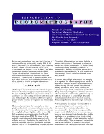
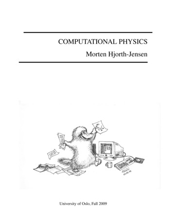
from pylab import *from scipy.integrate import odeint# plotting routines# routine for ODE integrationdef derivative(y, t):"""Right hand side of the differential equation.Here y [phi, v]."""return array([y[1], sin(y[0]) 0.25* cos(t)]) # (\dot{\phi}, \dot{v})def compute trajectory(y0):"""Integrate the ODE for the initial point y0 [phi 0, v 0]"""t arange(0.0, 100.0, 0.1)# array of timesy t odeint(derivative, y0, t)# integration of the equationreturn y t[:, 0], y t[:, 1]# return arrays for phi and v# compute and plot for two different initial conditions:phi a, v a compute trajectory([1.0, 0.9])phi b, v b compute trajectory([0.9, 0.9])plot(phi a, v a)plot(phi b, v b, "r-–")xlabel(r" \varphi ")ylabel(r"v")show()Figure 1. Python program to compute and visualize a driven pendulum’s time evolution.languages to be rather diverse, ranging from noexperience at all to detailed expertise in C .With a few exceptions, we rarely found previousknowledge of Python. To provide the necessarybasics, we give a short introduction to the language, which makes extensive use of Python’s interactive capabilities (with IPython). Thisintroduction covers the use of variables, simplearithmetic, loops, conditional execution, smallprograms, and subroutines. Of particular importance for numerical computations is the use of arrays provided by NumPy, which lets the studentswrite efficient code without explicit loops. Again,this makes the code compact but also enhances itsreadability and programming speed. Students canuse SciPy for additional numerical routines, suchas solving ordinary differential equations or computing special functions.Finally, we give a short introduction to plottingvia matplotlib. After starting IPython with supportfor interactive plotting via ipython –pylab, students can do# Array of x valuesx linspace(0.0, 2.0*pi, 100)# plot graph of sin(x) vs. x:MAY/JUNE 2007Figure 2. Pendulum example. Using matplotlib,we can visualize a driven pendulum’s dynamics(described in Equation 1) for two different initialconditions (bold and dashed curves).plot(x,sin(x))# add another graphplot(x,cos(2*x))and then zoom into the resulting plot via the mouse.31
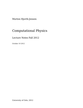
(a)(b)Figure 3. Isosurface example. The (a) screenshot of a MayaVi visualization shows a surface of constantvalue of n,l,m(x, y, z) 2 for the hydrogen atom, where n, l, m 5, 2, 1. With minor variations, we get(b) the same type of plot, but with a scalar cut-plane and a different lookup table.Two Examplesguerre polynomial (determined from scipy.A typical example we use in the classroom is a driven pendulum, described byspecial.assoclaguerre).ϕ sin ϕ (1 / 4 )cos t ,which we can rewrite as a coupled differentialequation:ϕ vυ sin ϕ (1 / 4 )cos t(1)for which the simple program in Figure 1 computesthe time evolution.Figure 2 shows the resulting plot of v versus asa screenshot; in this system, we see how a moderate change in the initial condition leads to quite different behavior after a short time period.A more advanced example is the visualization ofquantum probability densities for the hydrogenatom’s wave functions, which, in spherical coordinates, readsΨ n, l , m ( r , υ , ϕ ) Ylm (υ, ϕ ) ( n l 1)!( 2 / n )32n[( n l )]! ( 2r / n ) l e r / n L2nl l1 1 ( 2r / n ),(2)where n, l, and m are the quantum numbers thatcharacterize the wave function, Y is the sphericalharmonics (numerically determined from scipy.special.sphharm), and L is the associated La-32Because (x, y, z) is a scalar function defined on 3, we can either use a density plot or plot equienergy surfaces. Instead of writing the corresponding (nontrivial) visualization routines fromscratch, we use the extremely powerful Visualization Toolkit (VTK; www.vtk.org), whose routinesare also accessible from Python. The first step is togenerate a data file suitable for VTK by choosing arasterization in Cartesian coordinates (x, y, z) on[–40, 40]3 with 100 points in each direction,# vtk DataFile Version 2.0data.vtk hydrogen wave function dataASCIIDATASET STRUCTURED POINTSDIMENSIONS 100 100 100ORIGIN -40.0 -40.0 -40.0SPACING 0.8 0.8 0.8POINT DATA 1000000SCALARS scalars floatLOOKUPTABLE default. 1000000 real numbers correspondingto \psi {5,2,1}(x,y,z) 2.We can visualize this data set with MayaVi bystarting at the shell promptmayavi -d data.vtk -m IsoSurface -m AxesThis command line reads the data file hdata.vtk,COMPUTING IN SCIENCE & ENGINEERING
loads the isosurface module, and adds axes to theplot. By modifying the isosurface’s value, we get theplot in Figure 3a for n, l, m 5, 2, 1. Adding ascalar-cut-plane, a different color lookup table, andvarying the view takes us to Figure 3b. This shortexample shows that with only a moderate level ofeffort, highly instructive and appealing data visualizations are possible.At the end of the course, students give a shortpresentation on a small project of their choice. Inthis task, the students’ creativity isn’t limited byPython because it helps them create highly illustrative dynamical visualizations, some of them evenin 3D (with VPython; www.vpython.org).Our initial attempt at using Python forteaching computational physics hasproven to be highly successful. In fact,several students have continued to usePython for other tasks, such as data analysis in experimental physics courses or during a diplomathesis outside our group. The plan is to fully integrate the computational physics course into thecompulsory curriculum.AcknowledgmentsI thank Roland Ketzmerick, with whom the concept ofthis computational physics course was developed jointly.I also thank the people involved in setting up and runningthe course. Finally, a big thanks to all the authors andcontributors to Python and the software mentioned here.Arnd Bäcker is a scientific researcher at the Institut fürTheoretische Physik, Technische Universität Dresden. Hisresearch interests include nonlinear dynamics, quantumchaos, and mesoscopic systems. Bäcker has a PhD in theoretical physics from the Universität Ulm. Contact him atbaecker@physik.tu-dresden.de.AAPT Topical ConferenceComputational Physicsfor Upper Level Courses27–28 July 2007Davidson CollegeDavidson, NCFor further information go to www.opensourcephysics.org/CPCThe purpose of this conference is to identify problems where computation helps students understand key physicsconcepts. Participants are university and college faculty interested in integrating computation at their homeinstitutions. Some participants already teach or have taught computational physics to undergraduates and some arelooking for ways to integrate computational physics into their existing physics curriculum.Participants will contribute and discuss algorithms and curricular material for teaching core subjects such asmechanics, electricity and magnetism, quantum mechanics, and statistical and thermal physics. Participants willprepare and edit their material for posting on an AAPT website such as ComPADRE. Visiting experts will give talkson how computational physics may be used to present key concepts and current research to undergraduates.Participants are invited to prepare a poster describing how they incorporate computational physics into theirteaching, what projects they have assigned to students at different levels, and how computation has enhanced theircurriculum. Posters will remain up throughout the conference.Invited speakers include Amy Bug (Swarthmore College), Norman Chonacky (CiSE editor), Francisco Esquembre(University of Murcia, Spain), Robert Swendsen(Carnegie-Mellon University) , Steven Gottlieb (Indiana University),Rubin Landau (Oregon State University), Julien C. Sprott (University of Wisconsin), Angela Shiflet (Wofford College), and Eric Warren (Evernham Motorsports).The organizing committee consists of Wolfgang Christian, Jan Tobochnik, Rubin Landau, and Robert Hilborn.*Partial funding for this conference is being provided by Computing in Science & Engineering,the Shodor Foundation, the TeraGrid project, and NSF grant DUE-442581.MAY/JUNE 200733
PYTHON:BATTERIES INCLUDEDPython Unleashed on Systems BiologyResearchers at Cornell University have built an open source software system to modelbiomolecular reaction networks. SloppyCell is written in Python and uses third-partylibraries extensively, but it also does some fun things with on-the-fly code generation andparallel programming.Acentral component of the emergingfield of systems biology is the modelingand simulation of complex biomolecular networks, which describe the dynamics of regulatory, signaling, metabolic, anddevelopmental processes in living organisms. (Figure 1 shows a small but representative example ofsuch a network, describing signaling by G proteincoupled receptors.1 Other networks under investigation by our group appear online at www.lassp.cornell.edu/sethna/GeneDynamics/.) Naturally,tools for inferring networks from experimentaldata, simulating network behavior, estimatingmodel parameters, and quantifying model uncertainties are all necessary to this endeavor.Our research into complex biomolecular networks has revealed an additional intriguing property—namely, their sloppiness. These networks arevastly more sensitive to changes along some directions in parameter space than along others.2–5 Although many groups have built tools for simulatingbiomolecular networks (www.sbml.org), none sup-1521-9615/07/ 25.00 2007 IEEECopublished by the IEEE CS and the AIPCHRISTOPHER R. MYERS, RYAN N. GUTENKUNST,AND JAMES P. SETHNACornell University34THIS ARTICLE HAS BEEN PEER-REVIEWED.port the types of analyses that we need to unravelthis sloppiness phenomenon. Therefore, we’ve implemented our own software system—calledSloppyCell—to support our research (http://sloppycell.sourceforge.net).Much of systems biology is concerned with understanding the dynamics of complex biologicalnetworks and in predicting how experimentalinterventions (such as gene knockouts or drug therapies) can change that behavior. SloppyCell augments standard dynamical modeling by focusing oninference of model parameters from data and quantification of the uncertainties of model predictionsin the face of model sloppiness, to ascertain whethersuch predictions are indeed testable.The Python ConnectionSloppyCell is an open source software system written in Python to provide support for model construction, simulation, fitting, and validation. Oneimportant role of Python is to glue together manydiverse modules that provide specific functionality. We use NumPy (www.scipy.org/NumPy) andSciPy (www.scipy.org) for numerics—particularly,for integrating differential equations, optimizingparameters by least squares fits to data, and analyzing the Hessian matrix about a best-fit set of parameters. We use matplotlib for plotting (http://matplotlib.sourceforge.net). A Python interface tothe libSBML library (http://sbml.org/software/libsCOMPUTING IN SCIENCE & ENGINEERING
bml/) lets us read and write models in a standardized, XML-based file format, the Systems BiologyMarkup Language (SBML),6 and we use the pypar wrapper (http://datamining.anu.edu.au/ ole/pypar/) to the message-passing interface (MPI)library to coordinate parallel programs on distributed memory clusters. We can generate descriptions of reaction networks in the dot graphspecification language for visualization viaGraphviz (www.graphviz.org). Finally, we use thesmtplib module to have simulation runs sendemail with information on their status (for thosededicated researchers who can’t bear to be apartfrom their work for too long).Although Python serves admirably as the glue,we focus here on a few of its powerful features—the ones that let us construct highly dynamic andflexible simulation tools.GTPRRR GDPGDP GDP GTP GDPGTPCode Synthesisand Symbolic ManipulationResearchers typically treat the dynamics of reaction networks as either continuous and deterministic (modeling the time evolution ofmolecular concentrations) or as discrete and stochastic (by simulating many individual chemicalreactions via Monte Carlo). In the former case,we construct systems of ordinary differentialequations (ODEs) from the underlying networktopology and the kinetic forms of the associatedchemical reactions. In practice, these ODEs areoften derived by hand, but they need not be: allthe information required for their synthesis isembedded in a suitably defined network, but thestructure of any particular model is known onlyat runtime once we create and specify an instanceof a Network class.With Python, we use symbolic expressions (encoded as strings) to specify the kinetics of differentreaction types and then loop over all the reactionsdefined in a given network to construct a symbolicexpression for the ODEs that describe the timeevolution of all chemical species. (We depict the reactions as arrows in Figure 1; we can query each reaction to identify those chemicals involved in thatreaction [represented as shapes], as well as an expression for the instantaneous rate of the reactionbased on model parameters and the relevant chemical concentrations.) This symbolic expression isformatted in such a way that we can define a newmethod, get ddv dt(y, t), which is dynamicallyattached to an instance of the Network class usingthe Python exec statement. (The term “dv” in themethod name is shorthand for “dynamical variables”—that is, those chemical species whose timeMAY/JUNE 2007 GDPGTPFigure 1. Model for receptor-driven activation of heterotrimeric Gproteins.1 The signaling protein is inactive when bound toguanosine diphosphate (GDP) and active when bound toguanosine triphosphate (GTP). After forming a complex with a protein, binding to the active receptor R allows the protein torelease its GDP and bind GTP. The complex then dissociates into R, , and activated . The activated protein goes on to signaldownstream targets, whereas the protein is free to bring newinactive to the receptor.evolution we’re solving for.) We then use this dynamically generated method in conjunction withODE integrators (such as scipy.integrate.odeint, which is a wrapper around the venerableLSODA integrator,7,8 or with the variant LSODAR,9which we’ve wrapped up in SloppyCell to integrateODEs with defined events). We refer to thisprocess of generating the set of ODEs for a modeldirectly from the network topology as “compiling”the network.This sort of technique helps us do more than justsynthesize ODEs for the model itself. Similar techniques let us construct sensitivity equations for agiven model, so that we can understand how modeltrajectories vary with model parameters. To accomplish this, we developed a small package thatsupports the differentiation of symbolic Pythonmath expressions with respect to specified variables,35
by converting mathematical expressions to abstractsyntax trees (ASTs) via the Python compiler module. This lets us generate another new method,get d2dv dovdt(y, t), which describes the derivatives of the dynamical variables with respect toboth time and optimizable variables (model parameters whose values we’re interested in fitting todata). By computing parametric derivatives analytically rather than via finite differences, we can better navigate the ill-conditioned terrain of thesloppy models of interest to us.The ASTs we use to represent the detailed mathematical form of biological networks have otherbenefits as well. We also use them to generateLaTeX representations of the relevant systems ofequations—in practice, this not only saves us fromerror-prone typing, but it’s also useful for debugging a particular model’s implementation.Colleagues of ours who are developingPyDSTool (http://pydstool.sourceforge.net)—aPython-based package for simulating and analyzing dynamical systems—have taken this type of approach to code synthesis for differential equationsa step further. The approach we described earlierinvolves generating Python-encoded right-handsides to differential equations, which we use in conjunction with compiled and wrapped integrators.For additional performance, PyDSTool supportsthe generation of C-encoded right-hand sides,which it can then use to dynamically compile andlink with various integrators using the Pythondistutils module.Parallel Programming in SloppyCellBecause of the sloppy structure of complex biomolecular networks, it’s important not to just simulate a model for one set of parameters but to do soover large families of parameter sets consistent withavailable experimental data. Accordingly, we useMonte Carlo sampling to simulate a model withmany different parameter sets and thus estimate themodel uncertainties (error bars) associated withpredictions. Parallel computing on distributedmemory clusters efficiently enables these sorts ofextensive parameter explorations. Moreover, several different Python packages provide interfacesto MPI libraries, and we’ve found pypar to be especially useful in this regard.Whereas message passing on distributed memory machines is inherently somewhat cumbersomeand low level, pypar raises the bar by exploitingbuilt-in Python support for the pickling of complexobjects. Message passing in a low-level programming language such as Fortran or C typically requires constructing appropriately sized memory36buffers into which we must pack complex datastructures, but pypar uses Python’s ability to serialize (or pickle) an arbitrary object into a Pythonstring, which can then be passed from one processor to another and unpickled on the other side.With this, we can pass lists of parameters, modeltrajectories returned by integrators, and so on; wecan also send Python exception objects raised byworker nodes back to the master node for furtherprocessing. (These can arise, for example, if theODE integrator fails to converge for a particularset of parameters.)Additionally, Python’s built-in eval statementmakes it easy to create a very flexible worker thatcan execute arbitrary expressions passed as stringsby the master (requiring only that the inputs andreturn value are pickle-able). The following codesnippet demonstrates a basic error-tolerantmaster–worker parallel computing environmentfor arbitrarily complex functions and argumentsdefined in some hypothetical module namedour science:import pypar# our science contains the functions# we want to executeimport our scienceif pypar.rank() ! 0:# The workers execute this loop.# (The master has rank 0.)while True:# Wait for a message from# the master.msg pypar.receive(source 0)# Exit python if sent a# SystemExit exceptionif isinstance(msg, SystemExit):sys.exit()# Evaluate the message and# send the result back to# the master.# If an exception was raised,# send that instead.command, msg locals msglocals().update(msg locals)try:result eval(command)except X:result Xpypar.send(result, 0)# The code below is only run byCOMPUTING IN SCIENCE & ENGINEERING
# the master.# Evaluate our science.foo(bar) on each# worker, getting values for bar from# our science.todo.command ‘our science.foo(bar)’for worker in range(1, pypar.size()):args {‘bar’: \our science.todo[worker]}pypar.send((command, args), worker)# Collect results from all workers.results [pypar.receive(worker) \for worker in \range(1, pypar.size())]# Check if any of the workers failed.# If so, raise the resulting Exception.for r in results:if isinstance(r, Exception):raise r# Shut down all the workers.for worker in range(1, pypar.size()):pypar.send(SystemExit(), worker)We’ve very briefly described a fewof the fun and flexible featuresthat Python provides to supportthe construction of expressivecomputational problem-solving environments, suchas those needed to tackle complex problems in systems biology. Although any programming languagecan be coaxed into doing what’s desired with sufficient hard work, Python encourages researchers toask questions that they might not have even considered in less expressive environments.AcknowledgmentsWe thank Fergal Casey, Joshua Waterfall, RobertKuczenski, and Jordan Atlas for their help in developingand testing SloppyCell, and we acknowledge the insightsof Kevin Brown and Colin Hill in developing predecessorcodes, which have helped motivate our work.Development of SloppyCell has been supported by NSFgrant DMR-0218475, USDA-ARS project 1907-21000017-05, and an NIH Molecular Biophysics Training grantto Gutenkunst (no. T32-GM-08267).References1. V.Y. Arshavsky, T.D. Lamb, and E.N. Pugh, “G Proteins and Phototransduction,” Ann. Rev. Physiology, vol. 64, no. 1, 2002, pp.153–187.MAY/JUNE 20072. K.S. Brown and J.P. Sethna, “Statistical Mechanical Approachesto Models with Many Poorly Known Parameters,” Physical Rev.E, vol. 68, no. 2, 2003, p. 021904; http://link.aps.org/abstract/PRE/v68/e021904.3. K.S. Brown et al., “The Statistical Mechanics of Complex Signaling Networks: Nerve Growth Factor Signaling,” Physical Biology,vol. 1, no. 3, 2004, pp. 184–195; http://stacks.iop.org/14783975/1/184.4. J.J. Waterfall et al., “Sloppy-Model Universality Class and the Vandermonde Matrix,” Physical Rev. Letters, vol. 97, no. 15, 2006,pp. 150601–150604; http://link.aps.org/abstract/PRL/v97/e150601.5. R.N. Gutenkunst et al., “Universally Sloppy Parameter Sensitivities in Systems Biology,” 2007; http://arxiv.org/q-bio.QM/0701039.6. M. Hucka et al., “The Systems Biology Markup Language (SBML):A Medium for Representation and Exchange of Biochemical Network Models,” Bioinformatics, vol. 19, no. 4, 2003, pp. /cgi/content/abstract/19/4/524.7. A.C. Hindmarsh, “Lsode and Lsodi, Two New Initial Value Ordinary Differential Equation Solvers,” ACM-SIGNUM Newsletter, vol.15, no. 4, 1980, pp. 10–11.8. L.R. Petzold, “Automatic Selection of Methods for Solving Stiffand Nonstiff Systems of Ordinary Differential Equations,” SIAMJ. of Scientific and Statistical Computing, vol. 4, no. 1, 1983, pp.137–148.9. A.C. Hindmarsh, “Odepack, A Systematized Collection of ODESolvers,” Scientific Computing, North-Holland, 1983, pp. 55–64.Christopher R. Myers is a senior research associate andassociate director in the Cornell Theory Center at CornellUniversity. His research interests lie at the intersection ofphysics, biology, and computer science, with particularemphases on biological information processing, robustness and evolvability of natural and artificial networks,and the design and development of software systems toprobe complex spatiotemporal phenomena. Myers has aPhD in physics from Cornell. Contact him at myers@tc.cornell.edu; www.tc.cornell.edu/ myers.Ryan N. Gutenkunst is a graduate student in the Laboratory of Atomic and Solid State Physics at Cornell University. He uses SloppyCell to study universal properties ofcomplex biological networks, and is interested in howthese properties affect both practical model developmentand the dynamics of evolution. Gutenkunst has a BS inphysics from the California Institute of Technology. Contact him rng7@cornell.edu; http://pages.physics.cornell.edu/ rgutenkunst/.James P. Sethna is a professor of physics at Cornell University, and is a member of the Laboratory of Atomic andSolid State Physics. His recent research interests includecommon, universal features found in nonlinear optimization problems with many parameters, such as sloppymodels arising in the study of biological signal transduction. Sethna has a PhD in physics from Princeton University. Contact him at sethna@lassp.cornell.edu; www.lassp.cornell.edu/sethna.37
PYTHON:BATTERIES INCLUDEDReaching for the Stars with PythonThe author describes how Python has helped scientists calibrate and analyze data from theHubble Space Telescope, first as a means of scripting legacy applications, and, morerecently, as a way of developing new applications in Python itself.The Hubble Space Telescope (HST), a2.4-meter optical, ultraviolet, and infrared telescope, has orbited Earth formore than 16 years. Ground-basedtelescopes suffer the effects of the atmosphere. Inparticular, the atmosphere blurs the image, blocksultraviolet and infrared photons, and scatterslight—whether from the moon or your local streetlight—resulting in brighter backgrounds andgreater difficulty in observing faint sources. Beingabove the atmosphere means that the HST makessharper images of fainter sources at wavelengths notvisible from the ground. As a result, the HST canobtain exquisite observations and make many important discoveries that are otherwise unobtainable.The Space Telescope Science Institute (STScI) isresponsible for the HST’s scientific operation, including scheduling observations and processing anddisseminating the resulting data to both the publicand astronomers. Our group at STScI develops thesoftware used to calibrate and analyze the data. Thisarticle describes our experiences with the Python language and how we’ve incorporated it into our work.1521-9615/07/ 25.00 2007 IEEECopublished by the IEEE CS and the AIPPERRY GREENFIELDSpace Telescope Science Institute38THIS ARTICLE HAS BEEN PEER-REVIEWED.Using PythonOur initial use of Python was in developing an alternate scripting environment for a popular astronomical analysis system called IRAF (for ImagingReduction and Analysis Facility), which has its owncustom compiled language for its applications andits own scripting language and command-line environment. Although IRAF had great initial successand longevity (the US National Optical AstronomyObservatory developed it in the early 1980s), it hasproved to be an increasingly constrained development environment as time goes on. To remedy thissituation, we developed a way to script IRAF applications using Python so that we could run IRAFtasks more robustly and combine them with thewide variety of libraries and tools available inPython. This new scripting environment—calledPyRAF—proved easier to develop in Python thanwe expected and let us add more powerful capabilities than we had originally hoped (see s/white/pyrafpaper.pdf). Python had fewer limits onwhat it could accomplish—outside of efficiency concerns—and offered broad library support, powerfulyet easy-to-read language features (particularly itsnumerous language hooks for extending features tonew objects), and the ability to call out to C whennecessary (for which the need was rare). More important, Python’s interactive nature made it mucheasier to prototype, test, and debug applications.COMPUTING IN SCIENCE & ENGINEERING
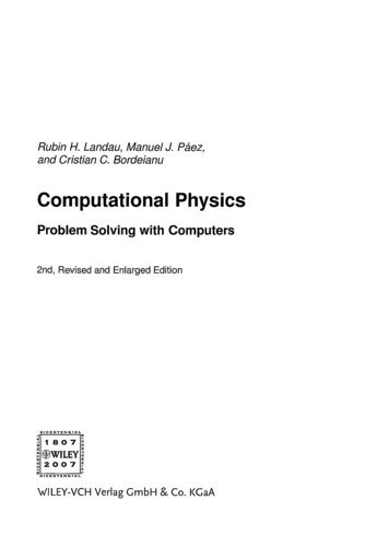
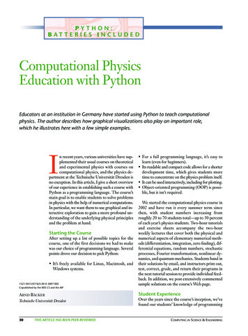
Figure 1. One raw exposure of the Tadpole galaxy (UGC10214). Each raw exposure consists of two 4,096 2,048 pixelcharge-coupled device images (one of which is shown). This 840-second exposure was taken with a wide-band filtercentered at 606 nm (orange-red). Most of the tens of thousands of star-like images, specks, and streaks aren’t stars—they’re the result of cosmic rays, and thus don’t represent detected photons. This figure (and Figure 2) uses a nonlinearintensity transfer function to emphasize the fainter features in the image.Because of our success with PyRAF, we decided todevelop as many of our applications in Python as possible. This seemed realistic because many astronomers have successfully developed useful toolsand applications with the commercial imageprocessing package IDL (Interactive Data Language), an interactive array manipulation languag
computational physics, and the physics de-partment at the Technische Universität Dresden is no exception. In this article, I give a short overview of our experience in establishing such a course with Python as a programming language. The course’s main goal is to enable students to solve problems i