Transcription
Fundamentals to BiostatisticsProf. Chandan ChakrabortyAssociate ProfessorSchool of Medical Science & TechnologyIIT Kharagpur
Statisticsdevelopment ofnew statisticaltheory &inferencecollection, analysis, interpretation of dataMath. StatisticsApplied StatisticsBiostatisticsstatistical methods are applied tomedical, health and biological dataapplication of themethods derived frommath. statistics tosubject specific areaslike psychology,economics and publichealthAreas of application of Biostatistics: Environmental Health, Genetics, Pharmaceutical research,Nutrition, Epidemiology and Health surveys etc
Some Statistical Tools for Medical DataAnalysis Data collection and Variables under study Descriptive Statistics & Sampling DistributionStatistical Inference – Estimation, Hypothesis Testing, Conf. Interval AssociationContinuous: Correlation and RegressionCategorical: Chi-square test Multivariate AnalysisPCA, Clustering Techniques, Discriminantion & Classification Time Series AnalysisAR, MA, ARMA, ARIMA
Population vs. SampleParameter vs. Statistics
Variable Definition: characteristic of interest in a study that has differentvalues for different individuals. Two types of variableContinuous: values form continuumDiscrete: assume discrete set of values ExamplesContinuous: blood pressureDiscrete: case/control, drug/placebo
Univariate Data Measurements on a single variable X Consider a continuous (numerical) variable Summarizing X– Numerically Center Spread– Graphically Boxplot Histogram6
Measures of center: Mean The mean value of a variable is obtained bycomputing the total of the values divided by thenumber of values Appropriate for distributions that are fairly symmetrical It is sensitive to presence of outliers, since all valuescontribute equally7
Measures of center: Median The median value of a variable is the numberhaving 50% (half) of the values smaller than it (andthe other half bigger) It is NOT sensitive to presence of outliers, since it‘ignores’ almost all of the data values The median is thus usually a more appropriatesummary for skewed distributions8
Measures of spread: SD The standard deviation (SD) of a variable is thesquare root of the average* of squared deviationsfrom the mean (*for uninteresting technical reasons,instead of dividing by the number of values n, youusually divide by n-1) The SD is an appropriate measure of spread whencenter is measured with the mean9
Quantiles The pth quantile is the number that has the proportionp of the data values smaller than it30%5.53 30th percentile10
Measures of spread: IQR The 25th (Q1), 50th (median), and 75th (Q3)percentiles divide the data into 4 equal parts; thesespecial percentiles are called quartiles The interquartile range (IQR) of a variable is thedistance between Q1 and Q3:IQR Q3 – Q1 The IQR is one way to measure spread when centeris measured with the median11
Five-number summary and boxplot An overall summary of the distribution of variablevalues is given by the five values:Min, Q1, Median, Q3, and Max A boxplot provides a visual summary of this fivenumber summary Display boxplots side-by-side to comparedistributions of different data sets12
BoxplotsuspectedoutliersQ3 whiskersmedianQ113
Histogram A histogram is a special kind of bar plot It allows you to visualize the distribution of values fora numerical variable When drawn with a density scale:– the AREA (NOT height) of each bar is the proportion ofobservations in the interval– the TOTAL AREA is 100% (or 1)14
Bivariate Data Bivariate data are just what they soundlike – data with measurements on twovariables; let’s call them X and Y Here, we are looking at two continuousvariables Want to explore the relationship betweenthe two variables15
Scatter plot We can graphically summarize a bivariate data setwith a scatter plot (also sometimes called a scatterdiagram) Plots values of one variable on the horizontal axisand values of the other on the vertical axis Can be used to see how values of 2 variables tendto move with each other (i.e. how the variables areassociated)16
Scatter plot: positive association17
Scatter plot: negative association18
Scatter plot: real data example19
Correlation Coefficient r is a unitless quantity -1 r 1 r is a measure of LINEAR ASSOCIATION When r 0, the points are not LINEARLYASSOCIATED – this does NOT mean there is NOASSOCIATION20
Breast cancer example Study on whether age at first child birth is an important riskfactor for breast cancer (BC)
Blood Pressure Example How does taking Oral Conceptive (OC) affect Blood Pressure (BP) in women paired samples
Birthweight Example Determine the effectiveness of drugA on preventing premature birth. Independent samples.
StatisticParameterMean:Xestimates Standarddeviation:sestimates Proportion:pestimates from samplefrom entirepopulation
PopulationMean, , isunknownSamplePoint estimate Interval estimateMean X 50I am 95%confident that is between40 & 60
Parameter Statistic Its Error
Sampling Distribution X or P X or P X or P
Standard ErrorSQuantitative VariableSE (Mean) np(1-p)Qualitative VariableSE (p) n
Confidence Intervalα/2α/21-α SESE95% Samples X- 1.96 SE X 1.96 SEZ-axisX
Confidence Intervalα/2α/21-α SESE95% Samplesp - 1.96 SEp 1.96 SEZ-axisp
Interpretation ofCIProbabilisticPracticalIn repeated sampling 100(1 )% of all intervals aroundsample means will in thelong run include We are 100(1- )%confident that the singlecomputed CI contains
Example (Sample size 30)An epidemiologist studied the bloodglucose level of a random sample of 100patients. The mean was 170, with a SD of10. X Z SESE 10/10 195%Then CI: 170 1.96 1168.04 171.96
Example (Proportion)In a survey of 140 asthmatics, 35%had allergy to house dust. Construct the95% CI for the population proportion.0.35(1- 0.04 p Z P(1-p) SE n0.35)1400.35 – 1.96 0.04 0.35 1.96 0.040.27 0.4327% 43%
Hypothesis testingA statistical method that usessample data toevaluate ahypothesis about a populationparameter. It is intended to helpresearchersdifferentiatebetween real and randompatterns in the data.
Null & Alternative Hypotheses H0 Null Hypothesis states theAssumption to be tested e.g. SBP ofparticipants 120(H0: 120). H1 Alternative Hypothesis is theopposite of the null hypothesis (SBP ofparticipants 120 (H1: 120). It may ormay not be accepted and it is thehypothesis that is believed to be trueby the researcher
Level of Significance, a Defines unlikely values of samplestatistic if null hypothesis is true.Called rejection region of samplingdistribution Typical values are 0.01, 0.05 Selected by the Researcher at theStart Provides the Critical Value(s) of theTest
Level of Significance, a and the RejectionRegionaRejectionRegions0CriticalValue(s)
Result PossibilitiesH0: InnocentHypothesis TestJury TrialActual SituationVerdictInnocentGuiltyActual SituationDecisionH 0 RejectH1- Type IError0FalsePositive( )H 0 FalseType IIError (b )Power(1 - b )FalseNegative
βFactors IncreasingType II Error True Value of Population Parameter– Increases When Difference BetweenHypothesized Parameter & True ValueDecreases Significance Level – Increases When Decreases Population Standard Deviation – Increases When Increases Sample Size n– Increases When n Decreasesbdb b bn
p Value Test Probability of Obtaining a TestStatistic More Extreme or ) thanActual Sample Value Given H0 Is True Called Observed Level of Significance Used to Make Rejection Decision––If p value Do Not Reject H0If p value , Reject H0
Hypothesis Testing: StepsTest the Assumption that the true mean SBP ofparticipants is 120 mmHg.State H0H0 : m 120State H1H1 : m 120Choose 0.05Choose nn 100Choose Test:Z, t, X2 Test (or p Value)
Hypothesis Testing: StepsCompute Test Statistic (or compute P value)Search for Critical ValueMake Statistical Decision ruleExpress Decision
One sample-mean Test Assumptions– Population is normallydistributed t test statisticsample mean null value x 0t sstandard errorn
Example Normal Body TemperatureWhat is normal body temperature? Is itactually 37.6oC (on average)?State the null and alternative hypothesesH0: 37.6oCHa: 37.6oC
Example Normal Body Temp (cont)Data: random sample of n 18 normal 6.837.637.436.138.736.237.237.5Summarize data with a test 161t2.38samplemean null value x 0t sstandarderrornP0.029
STUDENT’S t DISTRIBUTION TABLEDegrees offreedom151017202425 Probability (p value)0.100.050.016.31412.706 02.7872.576
Example Normal Body Temp (cont)Find the p-valueDf n – 1 18 – 1 17From SPSS: p-value 0.029From t Table: p-value isbetween 0.05 and 0.01.Area to left of t -2.11 equalsarea to right of t 2.11.The value t 2.38 is betweencolumn headings 2.110& 2.898 intable, and for df 17, the pvalues are 0.05 and 0.01.-2.11 2.11t
Example Normal Body Temp (cont)Decide whether or not the result isstatistically significant based on the pvalueUsing a 0.05 as the level of significancecriterion, the results are statistically significantbecause 0.029 is less than 0.05. In other words,we can reject the null hypothesis.Report the ConclusionWe can conclude, based on these data, that themean temperature in the human populationdoes not equal 37.6.
One-sample test for proportion Involves categorical variables Fraction or % of population in a category Sample proportion (p) p X number of successesnsample size Test is called Z testwhere:p Z Z is computed value (1 ) π is proportion inpopulationn(null hypothesisCritical Values: 1.96 at α 0.05value)2.58 at α 0.01
Example In a survey of diabetics in a large city, itwas found that 100 out of 400 have diabeticfoot. Can we conclude that 20 percent ofdiabetics in the sampled population havediabetic foot. Test at the 0.05 significance level.
SolutionHo: π 0.20Z H1: π 0.200.25 – 0.200.20 (1- 0.20)400 2.50Critical Value: 1.96Decision:RejectReject.025.025-1.960 1.96ZWe have sufficient evidence to reject theHo value of 20%We conclude that in the population ofdiabetic the proportion who havediabetic foot does not equal 0.20
Example3. It is known that 1% of population suffers from aparticular disease. A blood test has a 97% chance toidentify the disease for a diseased individual, by alsohas a 6% chance of falsely indicating that a healthyperson has a disease.a. What is the probability that a random person has apositive blood test.b. If a blood test is positive, what’s the probability thatthe person has the disease?c. If a blood test is negative, what’s the probability thatthe person does not have the disease?
A is the event that a person has a disease. P(A) 0.01; P(A’) 0.99. B is the event that the test result is positive.– P(B A) 0.97; P(B’ A) 0.03;– P(B A’) 0.06; P(B’ A’) 0.94; (a) P(B) P(A) P(B A) P(A’)P(B A’) 0.01*0.97 0.99 * 0.06 0.0691 (b) P(A B) P(B A)*P(A)/P(B) 0.97* 0.01/0.0691 0.1403 (c) P(A’ B’) P(B’ A’)P(A’)/P(B’) P(B’ A’)P(A’)/(1P(B)) 0.94*0.99/(1-.0691) 0.9997
Normal Distributions Gaussian distribution1 ( x x ) 2 / 2 x 2p ( x) N ( , ) e2 xxxE ( x) x Mean Variance Central Limit Theorem says sums of random variables tendtoward a Normal distribution. Mahalanobis Distance:E[( x x )2 ] x 2r x x x
Multivariate Normal Density x is a vector of d Gaussian variablesp( x) N ( , ) 12 d / 2 1 / 21 ( x )T 1( x )e 2 E[ x] xp( x)dx E[( x )( x ) ] ( x )( x )T p( x)dx T Mahalanobis Distancer 2 ( x )T 1( x ) All conditionals and marginals are also Gaussian
Bayesian Decision MakingClassification problem in probabilistic termsCreate models for how features aredistributed for objects of different classesWe will use probability calculus to makeclassification decisions104
Lets Look at Just One FeatureRBCY Each object canbe associatedwith multiplefeatures We will look atthe case of justone feature fornowXWe are going to define two key concepts .105
The First Key ConceptFeatures for each class drawn from class-conditional probability distributions(CCPD)P(X Class1)P(X Class2)XOur first goal will be to model these distributions106
The Second Key ConceptWe model prior probabilities to quantify the expected a priori chance of seeinga classP(Class2) & P(Class1)107
But How Do We Classify? So we have priors defining the a priori probabilityof a classP(Class1), P(Class2) We also have models for the probability of afeature given each classP(X Class1), P(X Class2)But we want the probability of the class given a featureHow do we get P(Class1 X)?108
Bayes RuleEvaluateevidenceBelief beforeevidenceLikelihoodPriorP( Feature Class ) P (Class )P(Class Feature) P( Feature)PosteriorBelief afterevidenceEvidenceBayes, Thomas (1763) An essaytowards solving a problem in thedoctrine of chances. PhilosophicalTransactions of the Royal Society ofLondon, 53:370-418109
Bayes Decision RuleIf we observe an object with feature X, how do decide if the object isfrom Class 1?The Bayes Decision Rule is simply choose Class1 if:P(Class1 X ) P(Class 2 X )P ( X Class1) P( L1) P ( X Class 2) P( L 2) P( X )P( X )is thenumberP( X This Class1)sameP(Class1) onPboth( X sides!Class 2) P(Class 2)Copyright@SMST110
Discriminant FunctionWe can create a convenient representation of theBayes Decision RuleP ( X Class1) P (Class1) P ( X Class 2) P (Class 2)P ( X Class1) P (Class1) 1P ( X Class 2) P (Class 2)G ( X ) logP ( X Class1) P (Class1) 0P ( X Class 2) P (Class 2)If G(X) 0, we classify as Class 1111
Stepping backWhat do we have so far?We have defined the two components, class-conditional distributions andpriorsP(X Class1), P(X Class2)P(Class1), P(Class2)We have used Bayes Rule to create a discriminant function forclassification from these componentsG ( X ) logP ( X Class1) P(Class1) 0P ( X Class 2) P(Class 2)Given a new feature, X, we plugit into this equation and if G(X) 0 we classify as Class1112
Getting P(X Class) from Training SetP(X Class1)There are 13 datapointsOne Simple ApproachDivide X values into binsAnd then we simply countfrequenciesX7/133/132/131/130 11-33-55-7 7113
Class conditional from Univariate Normal Distribution1 ( x x ) 2 / 2 x 2p ( x) N ( , ) e2 xxxMean :E ( x) xVariance :E[( x x )2 ] x 2Mahalanobis Distance :x xr x114
We Are Just About There .We have created the class-conditional distributions and priorsP(X Class1), P(X Class2)P(Class1), P(Class2)And we are ready to plug these into our discriminant functionP( X Class1) P(Class1)G ( X ) log 0P( X Class 2) P(Class 2)But there is one more little complication .115
Multidimensional feature space ?So P(X Class) become P(X1,X2,X3, ,X8 Class)and our discriminant function becomesP ( X 1 , X 2 ,., X 7 Class1) P(Class1)G ( X ) log 0P( X 1 , X 2 ,., X 7 Class 2) P (Class 2)116
Naïve Bayes ClassifierWe are going to make the following assumption:All features are independent given the classP( X 1 , X 2 ,., X n Class) P( X 1 Class ) P( X 2 Class).P( X n Class)n P ( X i Class )i 1We can thus estimate individual distributions for eachfeature and just multiply them together!117
Naïve Bayes Discriminant FunctionThus, with the Naïve Bayes assumption, we can now rewrite, this:G ( X 1 ,., X 7 ) logP( X 1 , X 2 ,., X 7 Class1) P(Class1) 0P( X 1 , X 2 ,., X 7 Class 2) P (Class 2)As this:G ( X 1 ,., X 7P ( X Class1) P(Class1) ) log 0 P( X Class 2) P(Class2)ii118
Classifying Parasitic RBCIntensityHu’s momentsFractal dimensionXiEntropyHomogeneityP(Xi Malaria)P(Xi Malaria)CorrelationChromatin dotsPlug these and priors into the discriminant functionG ( X 1 ,., X 7P ( X Mito) P( Mito) ) log 0 P( X Mito) P( Mito)iiIF G 0, we predict that the parasite is from class Malaria119
How Good is the Classifier?The RuleWe must test our classifier on a different setfrom the training set: the labeled test setThe TaskWe will classify each object in the test setand count the number of each type of error120
Binary Classification ErrorsPredicted TruePredicted False True (Mito)False ( Mito)TPFNFPTNSensitivity TP/(TP FN)Specificity TN/(TN FP)Sensitivity– Fraction of all Class1 (True) that we correctly predicted at Class 1– How good are we at finding what we are looking for Specificity– Fraction of all Class 2 (False) called Class 2– How many of the Class 2 do we filter out of our Class 1 predictions121In both cases, the higher the better
Thank you
Solution Critical Value: 1.96 Decision: We have sufficient evidence to reject the Ho value of 20% We conclude that in the population of diabetic the proportion who have diabetic foot does not equal 0.20 0 Z Reject Reject.025 .025 2.50 H o: π 0.20