Transcription
Chapter 1 Basics and Statistics ofAnalytical BiochemistryBiochemistry and Molecular Biology (BMB)1.1 Biochemical Studies1.2 Units of Measurements1.3 Weak Electrolytes1.4 Buffer Solution1.6 Quantitative Biochemical Measurements1.7.1-1.7.2 Principle of Clinical Biochemical AnalysisOthers: Receiver Operating Characteristic Curve Diagnosis Sensitivity and Specificity1
Basic principles Molarity : Number of moles of the substances in 1dm3 of solution. One mole: equal to molecular mass of the substance Molecular mass:Da: daltonskDa: Kilodaltons 1000 DaMr: no unitRelative molecular mass the molecular mass of a substance relative to1/12 of the atomic mass of the 12C .2
Units for Different Concentrations1 mol l-33
Ion StrengthsReason of deviation:Presence of electrolytes will result inelectrostatic interaction with other ions andsolventsTotal ion charge in solutionΜ 1/2 *(c1z12 c1z12 . cnzn2)c1, c2, cn: concentrations of each ion in molarityz1, z2, zn: charge on the individual ion4
5
Activity and Activity CoefficientsActivity : the effective concentration in solutionAx [Concentration ] γxγx : Activity coefficient The coefficient establish the relationship between activityand concentration. It will decrease when the ionic strength increases(include concentration, charge and ion mobility)e.g. 0.001 M Mg2 0.872Fe3 0.738Except for very diluted solution, the effective concentrationsare usually less than the actual concentration6
Preparation of Buffer SolutionOptimal enzyme activity pH 8α-Chymotrypsin:catalyzed cleavage of theC-N bond7
Henderson-Hasselbalch EquationFor a weak acid, which dissociates as follows:HA H A-log10Ka log10[H ] log10[A- ] - log10[HA]-log10[H ] -log10Ka log10[A-] - log10[HA]8
Why is pKa useful?Perhaps it is useful to look at this in another way: ifwe consider the situation where the acid is onehalf dissociated, in other words where [A-] isequal to [HA], then, substituting in theHenderson-Hasselbalch EquationpH pKa log10(1)pH pKa 0pH pKaThis means that an acid is halfdissociated when the pH of thesolution is numerically equal to thepKa of the acid.9
HA H A-Acids with the lowest pKavalues are able todissociate in solutions oflow pH, i.e. even where thehydrogen ion concentrationis high.Acids with higher pKavalues dissociate only insolutions of high (morealkaline) pH.10
11
Quantitative BiochemicalMeasurements What to study?Model How to studyMethod Is the results correct?Performance How to interpret results?Report12
Quantitative BiochemicalMeasurements Analytical Considerations:(I) Test Model :in vivo v.s. in vitroMaterial: urine, serum/plasma/bloodMatrix v.s AnalyteSampling v.s population13
in vivo v.s. in vitroIn vivo:In a living cell or organismBiological or chemical workdoneinthetesttube(in glass)In vitro:14
Sampling v.s PopulationPopulation: Representative portion of analyteHeterogeneous v.s HomogeneousExtraction Methods: Liquid extraction Solid-phase extraction Laser microdisection(cancer cell) .etc15
Quantitative Biochemical Measurements(II) Selection of Analytical Methods Qualitative v.s Quantitative analysis Chemical and physical properties ofanalyte Precision, accuracy and detection limit Interference from matrix Cost and value Possible hazard and riskNOTE16
Precision v.s. Accuracy forQuantitative or Numerical dataAccuracy— a measure of rightness.Accuracy can be defined how closely a measuredvalue agrees with the correct value.Accuracy is determined by comparing a number to aknown or accepted value.Precision — a measure of exactness.Precision can be defined how closely individualmeasurements agree with each other.It is sometimes defined as reproducibility17
Accuracy Precision Accuracy Precision XThe average is closeto the center but theindividual values arenot similarAccuracy PrecisionX Accuracy PrecisionXX18
Physical Basis of Analytical MethodsPhysical properties that Examples of properties used in thecan be measured withProteinLeadOxygensome degree of precisionExtensiveMassVolumeMechanicalSpecific gravityViscositySurface alf-cell potentialNuclearRadioactivity 19
Major manipulative steps in a generalizedmethod of analysisPurification of the test substance Development of a physical characteristic by the formation of aderivative Detection of an inherent or induced physical characteristic Signal amplification Signal measurement Computation Presentation of result20
Quantitative BiochemicalMeasurements(III) Experimental Errors Systematic error Random errorStandard Operation Procedures(SOP)21
Systematic Error Constant or proportional (Bias) Also calledOverestimation /underestimation(1) Analyst error: pipette, calibration, solutionpreparation, method design(2) Instrumental error: contamination ofinstrument, power fluctuation, variation in T,pH, electronic noise(3) Method error: side reaction, incompletereaction22
Identification of Systematic Errors Blank sampleStandard reference sampleAlternative methodsExternal quality assessment sample23
Random Error Variable, either positive or negative also calledIndeterminate error(1) Instrumental error: random electric noise24
Standard Operating Procedures(SOP)Detailed, written instructions to achieve uniformityof the performance of a specific process;Include: Quantity/quality of reagent Preparation of standard solution Calibration of instrument Methodology of actual analyticalprocedures25
Assessment of Performance ofAnalytical MethodQuestion:1.What is the correlation of the memory ofimmune cell and cancer metastasis?2.Will it affect the survival rate?(大腸直腸癌)NEJM, 353, 2654-2666, 200526
BackgroundThe role of tumor-infiltrating (浸潤) immune cells inthe early metastatic invasion (轉移性侵犯) ofcolorectal cancer (直腸癌) is unknown.MethodsWe studied pathological signs of early metastaticinvasion (venous emboli 靜脈栓塞 and lymphatic 淋巴 and perineural invasion(神經旁間隙) in 959specimens of resected colorectal cancer. The localimmune response within the tumor was studied byflow cytometry (39 tumors), low density-array realtime polymerase-chain-reaction assay (75 tumors),and tissue microarrays (415 tumors).27
Disease-free survival5 yr Median P%mo valueOverall survival Disease-free survival (DFS) denotes the chancesof staying free of disease after a particular treatment for agroup of individuals suffering from a cancer. Overall survival is a term that denotes the chancesof staying alive for a group of individuals suffering from a28cancer.
VELIPI (早期轉移)---early steps of themetastatic processes,which include vascular emboli,lymphatic invasion,and perineural invasion.Relapse復發29
Interpretation of Quantitative DataIs the difference of measured mean valuesfrom the two groups significantly different ?30
How do we evaluate the data ?Are the two groups different?Normal control (健康) 52 54 Cancer Patient (癌症)31
Normal v.s Patient?A. Discrimination - Comparison of DataGroups1. 2 groups with equal variances2. 2 groups with unique variancesB. Receiving Operating Characteristic (ROC)curve1.2.3.4.2 X 2 contingency tablesensitivity & specificityplotting ROC curveuses of ROC curve32
When the two study groups do havestatistically significant difference, howdo we evaluate the correlation of anynew data with the two groups?33
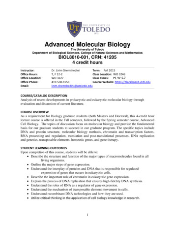
Receiver Operating Characteristics Curve(ROC curve analysis)The diagnostic performance of a test, or the accuracy of a test todiscriminate diseased cases from normal cases is evaluatedusing Receiver Operating Characteristic (ROC) curve analysisTN: true negativeFN: false negativeTP: true positiveFP: false positive
2 x 2 Contingency TableHealthyDiseaseHealthyabcdDiagnosis thresholdDiagnosis thresholdResultDiseaseDisease (true)TotalAbsent PresentNormal (negative)Disease (positive)totalaca cbdb da bc da b c dCorrectWrong35
36
NotumorTumor37
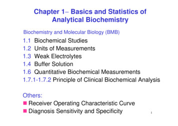
Receiver Operating Characteristics (ROC) CurveHigh noise,Lots of overlapLow noise,Not much overlap38
Sensitivity & Specificity Sensitivity probability that a test result will be positive when thedisease is present (true positive rate, expressed as apercentage).Sensitivity P(disease positive disease) d / (b d)– True Positive(1-sensitivity) : False Negative39
Sensitivity & Specificity Specificity probability that a test result will be negativewhen the disease is not present (true negativerate, expressed as a percentage) Specificity P(disease negative noraml) a / (a c)– True negative(1-specificity) : False positive40
Sensitivity and Specificity versusCriterion ValueWhen you select a higher criterion value, the false positive fractionwill decrease with increased specificity but on the other hand the truepositive fraction and sensitivity will decrease.When you select a lower criterion value, then the true positive fractionand sensitivity will increase. On the other hand the false positivefraction will also increase, and therefore the true negative fraction 41and specificity will decrease.
Plotting ROC CurveReceiver Operating Characteristics Curve Y軸:Sensitivity (true positive) X軸(1-specificity)(false positive)(normal, but wrong diagnosis)不同判定標準42
Uses of ROC curve to DetermineDiagnosis Threshold Area under Curve(AUC)– 0.9 1.0: excellent– 0.8 0.9: good– 0.7 0.8: fair– 0.6 0.7: poor– 0.5 0.6: worthless43
J Clin Epidemiol, Jul 1997;50(7):837-43BMI 20164 cm, 53 kgBMI :weight (Kg)/Height (m2)The ROC curve shows the trade-offsbetween Sensitivity and Specificity.This article‘s Authors believed that aBMI of 20.5 was the optimum thresholdto define obesity, with a Sensitivity of84% and Specificity of 60%. Can youbelieve it? A BMI of 20.5 to defineobesity (肥胖) ? What were theythinking?44
Assessment of the Performance of a Method(BMB 1.6.2)Summary Statistics Measures of Central Tendency– Mean, Median, Mode Spread–Range–Variance–Standard deviation–Stander error Shape45
Data Follows Normal Distribution1 x µ (1f ( x) e 22π σσ)2 The x-axis represents the values ofa particular variable The y-axis represents theproportion of members of thepopulation that have each value ofthe variable The area under the curverepresents probability – i.e. areaunder the curve between two valueson the x-axis represents theprobability of an individual having avalue in that range46
Real-World QuantificationConfidence Interval orZone of UncertaintyAccuracyPrecisionTrue mean Value47
'Student's' t TestThe t-test compares theactual differencebetween two means inrelation to the variationin the datahttp://www.socialresearchmethods.net/kb/stat t.htm48
'Student's' t Test One-sample t-test: know the mean differencebetween the sample and the known value of thepopulation mean. Unpaired t-test: compare two population means Paired t-test: compare the values of meansfrom two related samples, for example in a‘before and after’ scenario.When tcalc ttable ,the two value are notthe same (within the confidence intervals)49
Measures of Central e.g.510152025302, 5, 5, 7, 9, 11, 13, 22mode 5 (greatest frequency)median (7 9)/2 8mean (2 5 5 7 9 11 13 22)/8Median 0
Spread -----Variance Variance (變異數):n12s2 (x x) i(n 1) i 1 Standard Deviation, S.D. (標準差) gives the dispersion of numerical data aroundthe mean value :1n 12 s ( xi x ) (n 1) i 12N-1: degree of freedom [Number of observation 1]51
Q: Why do we divide by (n-1) and not by (n)? Use of n as a divisor will give a samplestandard deviation which tends tounderestimate the population standarddeviation, whereas the use of (n-1) giveswhat is known as an”unbiased estimator” Score deviates less from their own mean thanfrom any other number. So, the calculationsubtracting each score from the sample meanwill be smaller than subtracting form thepopulation mean------ underestimate the SD(n-1)Statistics for Analytical Chemists, by R. Caulcutt and R. Boddy52
Spread -----Coefficient of VarianceCoefficient of Variation (變異係數):Relative standard deviationsCV 100%xe.g. A: 2.00 0.10 mM, CV 5.0%B: 8.00 0.41 mM, CV 5.0%53
Spread -----Coefficient of Variance Possibility of occurrence80% Rainy98% Rainy, Cloudy, Sunny p-valueP 0.05 ( 95% confidence)-----Statistically significantµ x54
Define the spread or distribution ofthe data68.3% data will be within the range of X 1 S.D.The possibility of a data point within the range ofX 1 S.D. is 68.3%. 1 S.D. 2 S.D.Frequency ofoccurrence of ameasurement 3 S.D.Gaussian Distribution/Normal Distribution55
Example 556
Accuracy ( Bias, Inaccuracy)Differences between “mean” and “true” valuec When the number of sampling approaches infinity,“mean” is equal to the “population mean ”d If the “uncertainty” (SD) is close to 0,Then,n much approach infinity(Eg:when SD is 1/2 n has to increase to 4-fold)n 12 s ( xi x ) (n 1) i 1 12
How do we evaluate the differenceof measured “mean” and “truemean” of the population?In practical experimental design, it is notpossible to sample EVERY analyte from thepopulation.Animal model, cancer vs healthy group .etc58
Standard Error (of the mean, S.E.)363135PopulationS.D variability of original dataThe absolute value of S.D.can not tell the difference ofmean and popuation mean3239S.E35SD variability of meanN .Why does the denominator read N1/2 instead of just N?Because we are really dividing the variance, which is SD2,by N, but we end up again with squared units, so we takethe square root of everything .59
SD v.s. SE 12 s ( xi x ) (n 1) i 1nSE 12SDN60
Spread--Confidence IntervalGives a range of values about the sample meanwithin a given probability for normal distributionP( 1.96 z 1.96) 0.95 , and z P ( x 1.96σn µ x 1.96σnx µσ/ n) 0.95A confidence interval gives an estimated rangeof values which is likely to include an unknownpopulation parameter, the estimated rangebeing calculated from a given set of sample data61
Spread---Confidence IntervalThe lower and upper boundaries / values of a confidenceinterval, that is, the values which define the range of aconfidence intervalSD SD M X (t ) X - (t ) n n Confidence Limitt:student‘s factor (Table 1.9)X62
Example 6SD SD ()()XMXtt nn 63
OutlierRejection of outlier experimental data outlier outliersQ exp (Dixon’s Q-test)Experimental rejection quotientThe data point closest to analyteQ expX n - X n -1gap X n - X1range64
Outlier– Q valuesTable.1.1Values of Q for the rejection of outliersQ (95% conflidence)Number of observations40.8350.7260.6270.5780.52Qexp Q Table 1.10 ------ Accept the datapointQexp Q Table 1.10 ------ Reject the datapoint65
Example 766
‘Student’s‘ t Test— Test of e t-test compares the actualdifference between two meansrelative to the variation in thedata sample mean v.s.true meanDetermine whether a significantdifference exist between twomean or whether the twopopulation means are at t.htm
t value:.calculated by integrating the distributionbetween confident limitsstandard error ofthe difference68
The t-distribution In fact we have many t-distributions, each one iscalculated in reference to the number of degrees offreedom (d.f.) also know as variables (v)Normaldistributiont-distribution
Student’s t Values (Table 1.9)Table 1.9MBM, p38Values for Student's tConfidence Level (%)Degree 799.970
t-test InterpretationReject H0.025-2.0154Reject H0.025 (p)0 2.0154tNote as t increases, p decreasest (value) must t (critical on table) by P level
Finding a Critical t A .05A .05tc 1.812-tc -1.812Degrees of Freedom12.10The table provides the t values(tc) for which P(tx tc) 6531.6451.9721.962.3452.326 t.00563.6579.925.3.169.2.6012.576
One-Sample t-test Compare the result with the known value of the solutionoften test whether the mean of a variable is less than,greater than, or equal to a specific value.tSnM X t calc(M - X) nSKnown valueWhent calc 〉 t table(1.9) if S.E is not in the range of X XXThe result is not within the range of populationt calc 〉 t table(1.9)The result is consistent with the population73
Example 874
75
Unpaired Statistical ExperimentsConditionGroup 1members ConditionGroup 2membersOverall setting: 2 groups of 4 individuals each– Group1: TIGP students– Group2: NTU students Experiment 1:– We measure the height of all students– We want to establish if members of one group are consistently (or onaverage) taller than members of the other, and if the measureddifference is significant Experiment 2:– We measure the weight of all students– We want to establish if members of one group are consistently (or onaverage) heavier than the other, and if the measured difference issignificant Experiment 3:–
Unpaired Statistical Experiments In unpaired experiments, you typically have two groups ofpeople that are not related to one another, and measuresome property for each member of each group e.g. you want to test whether a new drug is effective or not,you divide similar patients in two groups:– One groups takes the drug– Another groups takes a placebo– You measure (quantify) effect of both groups some timelater You want to establish whether there is a significantdifference between both groups at that later point
Unpaired StatisticalExperiments1. How do we address theproblem?2. Compare two sets of results(alternatively calculate meanfor each group and comparemeans)1. Graphically:1. Scatter Plots2. Box plots, etc140120100806040200Are these two seriessignificantly different?140120100806040202. Compare Statistically1. Use unpaired t-test0Are these two seriessignificantly different?
Unpaired t-test: Are two data sets different ? applied to two independent groupse.g. diabetic patients versus nondiabetics sample size from the two groupsHomay or may not be equalPopulatioPopulation in addition to the assumption thatthe data is from a normal distribution,there is also the assumption that thestandard deviation (SD)s isapproximately the same in bothHaPopulation 1Population79
首先要比較2方法的標準差 (Similar ? Different?)F F-testS12S22 largest variationsmallest variation例:Group A mean:50 mg/l , n 5 , S 2.0mg/lB mean:45 mg/l , n 6 , S 1.5mg/lF 221.5 2 1.78Table1.1Degree of freedom at 95%:(n-1) (n2-1) (5-1) (6-1) 9Ftable 7.39 〉 Fcalc 1.78 the variance values are the same the mean really differs80
Similar S(With Equal Variances)‧equation 1.18、1.19tcalcµ1x1 x2 S pooledn1n2n1 n2µ2S pooledan estimator of the commonstandard deviation of the twosamples:S pooled s12 (n1 1) s22 (n2 1)n1 n2 2degree of freedom n1 n2 281
Different S (With Unequal Variances)This test is used only when the two samplesizes are unequal and the variance is assumedto be different.‧ equation 1.20、1.21tcalc x1 x2( s / n1 ) ( s / n2 )2122(1.18)(1.19) ( s12 / n1 s22 / n2 ) 2degree of freedom 2 2222 [( s1 / n1 ) /(n1 1)] [( s2 / n2 ) /(n2 1)] 或( s12 / n1 s22 / n2 ) 2[( s12 / n1 ) 2 /( n1 1)] [( s22 / n2 ) 2 /( n2 1)]82
Condition1Paired statistical experiments Condition2GroupmembersOverall setting: 1 groups of 4 individuals each– Group1: TIGP students– We make measurements for each student in two situations Experiment 1:– We measure the height of all students before Bioinformatics courseand after Bioinformatics course– We want to establish if Bioinformatics course consistently (or onaverage) affects students’ heights Experiment 2:– We measure the weight of all students before Bioinformatics courseand after Bioinformatics– We want to establish if Bioinformatics course consistently (or onaverage) affects students’ weights Experiment 3:–
Condition 1 Condition 2Paired statistical experimentsGroupmembers In paired experiments, you typically have one group of people, youtypically measure some property for each member before andafter a particular event (so measurement come in pairs of beforeand after) e.g. you want to test the effectiveness of a new cream for tanning– You measure the tan in each individual before the cream isapplied– You measure the tan in each individual after the cream isapplied You want to establish whether the there is a significant differencebetween measurements before and after applying the cream forthe group as a whole
Paired statistical experiments The WT/KO example is a paired experiment if the rats in theexperiments are the same!Experiments for Gene 96608 atRat #WT geneKO geneexpression expressionRat1100200Rat2100300Rat3200400Rat4300500
Paired statistical experiments151.2.3.4.How do we address the problem?Calculate difference for each pairCompare differences to zeroAlternatively (compare averagedifference to zero)5. Graphically:1. Scatter Plot of difference2. Box plots, etc6. Statistically1050-5-10-15Are differences close to Zero?151051. Use unpaired t-test0-5-10-15
Paired t-test Data is derived from study subjects who have beenmeasured at two time points (so each individual has twomeasurements). The two measurements generally arebefore and after a treatment interventionEg: control versus treated sample 95% confidence interval is derived from the differencebetween the two sets of paired observationsequation 1.22、1.23tcalc dsdnsd 2(d d) in 187
Example10COMPARISON OF TWO ANALYTICAL METHODS USINGDIFFERENT TEST SAMPLES88
answer89
tcalc tcalc(known value x ) nsx x 1 2S pooleds12 (n1 1) s22 (n2 1)n1 n2 2S pooled tcalc n1n2n1 n2x1 x2( s / n1 ) ( s / n2 )2122(1.17)(1.18)(1.19)(1.20) ( s12 / n1 s22 / n2 ) 2Degree of freedom 2 2222 [( s1 / n1 ) /(n1 1)] [( s2 / n2 ) /(n2 1)] tcalc sd dsdn (di(1.21)(1.22) d )2n 1(1.23)90
Chapter 1 Basics and Statistics of Analytical Biochemistry 1.1 Biochemical Studies 1.2 Units of Measurements 1.3 Weak Electrolytes 1.4 Buffer Solution 1.6 Quantitative Biochemical Measurements 1.7.1-1.7.2 Principle of Clinical Biochemical Analysis Others: Receiver Operating C