Transcription
Chapter 30Real-Time Simulation andRendering of 3D FluidsKeenan CraneUniversity of Illinois at Urbana-ChampaignIgnacio LlamasNVIDIA CorporationSarah TariqNVIDIA Corporation30.1 IntroductionPhysically based animation of fluids such as smoke, water, and fire provides some of themost stunning visuals in computer graphics, but it has historically been the domain ofhigh-quality offline rendering due to great computational cost. In this chapter we shownot only how these effects can be simulated and rendered in real time, as Figure 30-1demonstrates, but also how they can be seamlessly integrated into real-time applications. Physically based effects have already changed the way interactive environmentsare designed. But fluids open the doors to an even larger world of design possibilities.In the past, artists have relied on particle systems to emulate 3D fluid effects in real-timeapplications. Although particle systems can produce attractive results, they cannot matchthe realistic appearance and behavior of fluid simulation. Real time fluids remain a challenge not only because they are more expensive to simulate, but also because the volumetric data produced by simulation does not fit easily into the standard rasterization-basedrendering paradigm.30.1IntroductionFrom the new book GPU Gems 3, edited by Hubert Nguyen, published by Addison-Wesley Professional,August 2007, ISBN 0321515269. Copyright 2008 NVIDIA Corporation. For more information, please visit:www.awprofessional.com/title/0321515269.633
Figure 30-1. Water Simulated and Rendered in Real Time on the GPUIn this chapter we give a detailed description of the technology used for the real-timefluid effects in the NVIDIA GeForce 8 Series launch demo “Smoke in a Box” and discuss its integration into the upcoming game Hellgate: London.The chapter consists of two parts: Section 30.2 covers simulation, including smoke, water, fire, and interaction withsolid obstacles, as well as performance and memory considerations.Section 30.3 discusses how to render fluid phenomena and how to seamlessly integrate fluid rendering into an existing rasterization-based framework.30.2 Simulation30.2.1 BackgroundThroughout this section we assume a working knowledge of general-purpose GPU(GPGPU) methods—that is, applications of the GPU to problems other than conventional raster graphics. In particular, we encourage the reader to look at Harris’s chapteron 2D fluid simulation in GPU Gems (Harris 2004). As mentioned in that chapter,implementing and debugging a 3D fluid solver is no simple task (even in a traditionalprogramming environment), and a solid understanding of the underlying mathematics634Chapter 30Real-Time Simulation and Rendering of 3D FluidsCopyright NVIDIA Corporation. All rights reserved.
and physics can be of great help. Bridson et al. 2006 provides an excellent resource inthis respect.Fortunately, a deep understanding of partial differential equations (PDEs) is not required to get some basic intuition about the concepts presented in this chapter. AllPDEs presented will have the form x f ( x , t ), twhich says that the rate at which some quantity x is changing is given by some functionf, which may itself depend on x and t. The reader may find it easier to think about thisrelationship in the discrete setting of forward Euler integration:x n 1 x n f ( x n, t n ) Δt .In other words, the value of x at the next time step equals the current value of x plusthe current rate of change f (x n, t n) times the duration of the time step Δt. (Note thatsuperscripts are used to index the time step and do not imply exponentiation.) Bewarned, however, that the forward Euler scheme is not a good choice numerically—weare suggesting it only as a way to think about the equations.30.2.2 Equations of Fluid MotionThe motion of a fluid is often expressed in terms of its local velocity u as a function ofposition and time. In computer animation, fluid is commonly modeled as inviscid (thatis, more like water than oil) and incompressible (meaning that volume does not changeover time). Given these assumptions, the velocity can be described by the momentumequation: u1 (u ) u p f , tρsubject to the incompressibility constraint: u 0,where p is the pressure, ρ is the mass density, f represents any external forces (such asgravity), and is the differential operator: x yT . z 30.2Copyright NVIDIA Corporation. All rights reserved.Simulation635
To define the equations of motion in a particular context, it is also necessary to specifyboundary conditions (that is, how the fluid behaves near solid obstacles or other fluids).The basic task of a fluid solver is to compute a numerical approximation of u. Thisvelocity field can then be used to animate visual phenomena such as smoke particles ora liquid surface.30.2.3 Solving for VelocityThe popular “stable fluids” method for computing velocity was introduced in Stam 1999,and a GPU implementation of this method for 2D fluids was presented in Harris 2004.In this section we briefly describe how to solve for velocity but refer the reader to the citedworks for details.In order to numerically solve the momentum equation, we must discretize our domain(that is, the region of space through which the fluid flows) into computationalelements. We choose an Eulerian discretization, meaning that computational elementsare fixed in space throughout the simulation—only the values stored on these elementschange. In particular, we subdivide a rectilinear volume into a regular grid of cubicalcells. Each grid cell stores both scalar quantities (such as pressure, temperature, and soon) and vector quantities (such as velocity). This scheme makes implementation on theGPU simple, because there is a straightforward mapping between grid cells and voxelsin a 3D texture. Lagrangian schemes (that is, schemes where the computational elements are not fixed in space) such as smoothed-particle hydrodynamics (Müller et al.2003) are also popular for fluid animation, but their irregular structure makes themdifficult to implement efficiently on the GPU.Because we discretize space, we must also discretize derivatives in our equations: finitedifferences numerically approximate derivatives by taking linear combinations of valuesdefined on the grid. As in Harris 2004, we store all quantities at cell centers for pedagogical simplicity, though a staggered MAC-style grid yields more-robust finite differences and can make it easier to define boundary conditions. (See Harlow and Welch1965 for details.)In a GPU implementation, cell attributes (velocity, pressure, and so on) are stored inseveral 3D textures. At each simulation step, we update these values by running computational kernels over the grid. A kernel is implemented as a pixel shader that executes onevery cell in the grid and writes the results to an output texture. However, because636Chapter 30Real-Time Simulation and Rendering of 3D FluidsCopyright NVIDIA Corporation. All rights reserved.
GPUs are designed to render into 2D buffers, we must run kernels once for each sliceof a 3D volume.To execute a kernel on a particular grid slice, we rasterize a single quad whose dimensions equal the width and height of the volume. In Direct3D 10 we can directly renderinto a 3D texture by specifying one of its slices as a render target. Placing the slice indexin a variable bound to the SV RenderTargetArrayIndex semantic specifies theslice to which a primitive coming out of the geometry shader is rasterized. (See Blythe2006 for details.) By iterating over slice indices, we can execute a kernel over the entiregrid.Rather than solve the momentum equation all at once, we split it into a set of simpleroperations that can be computed in succession: advection, application of externalforces, and pressure projection. Implementation of the corresponding kernels is detailedin Harris 2004, but several examples from our Direct3D 10 framework are given inListing 30-1. Of particular interest is the routine PS ADVECT VEL: this kernel implements semi-Lagrangian advection, which is used as a building block for more accurateadvection in the next section.Listing 30-1. Simulation Kernelsstruct GS OUTPUT FLUIDSIM{// Index of the current grid cell (i,j,k in [0,gridSize] range)float3 cellIndex : TEXCOORD0;// Texture coordinates (x,y,z in [0,1] range) for the// current grid cell and its immediate neighborsfloat3 CENTERCELL : TEXCOORD1;float3 LEFTCELL: TEXCOORD2;float3 RIGHTCELL : TEXCOORD3;float3 BOTTOMCELL : TEXCOORD4;float3 TOPCELL: TEXCOORD5;float3 DOWNCELL: TEXCOORD6;float3 UPCELL: TEXCOORD7;float4 pos: SV Position; // 2D slice vertex in// homogeneous clip spaceuint RTIndex: SV RenderTargetArrayIndex; // Specifies// destination slice};30.2Copyright NVIDIA Corporation. All rights reserved.Simulation637
Listing 30-1 (continued). Simulation Kernelsfloat3 cellIndex2TexCoord(float3 index){// Convert a value in the range [0,gridSize] to one in the range [0,1].return float3(index.x / textureWidth,index.y / textureHeight,(index.z 0.5) / textureDepth);}float4 PS ADVECT VEL(GS OUTPUT FLUIDSIM in,Texture3D velocity) : SV Target{float3 pos in.cellIndex;float3 cellVelocity os - timeStep * cellVelocity;pos cellIndex2TexCoord(pos);return velocity.Sample(samLinear, pos);}float PS DIVERGENCE(GS OUTPUT FLUIDSIM in,Texture3D velocity) : SV Target{// Get velocity values from neighboring cells.float4 fieldL velocity.Sample(samPointClamp, in.LEFTCELL);float4 fieldR velocity.Sample(samPointClamp, in.RIGHTCELL);float4 fieldB velocity.Sample(samPointClamp, in.BOTTOMCELL);float4 fieldT velocity.Sample(samPointClamp, in.TOPCELL);float4 fieldD velocity.Sample(samPointClamp, in.DOWNCELL);float4 fieldU velocity.Sample(samPointClamp, in.UPCELL);// Compute the velocity’s divergence using central differences.float divergence 0.5 * ((fieldR.x - fieldL.x) (fieldT.y - fieldB.y) (fieldU.z - fieldD.z));return divergence;}638Chapter 30Real-Time Simulation and Rendering of 3D FluidsCopyright NVIDIA Corporation. All rights reserved.
Listing 30-1 (continued). Simulation Kernelsfloat PS JACOBI(GS OUTPUT FLUIDSIM in,Texture3D pressure,Texture3D divergence) : SV Target{// Get the divergence at the current cell.float dC divergence.Sample(samPointClamp, in.CENTERCELL);// Get pressure values from neighboring cells.float pL pressure.Sample(samPointClamp, in.LEFTCELL);float pR pressure.Sample(samPointClamp, in.RIGHTCELL);float pB pressure.Sample(samPointClamp, in.BOTTOMCELL);float pT pressure.Sample(samPointClamp, in.TOPCELL);float pD pressure.Sample(samPointClamp, in.DOWNCELL);float pU pressure.Sample(samPointClamp, in.UPCELL);// Compute the new pressure value for the center cell.return(pL pR pB pT pU pD - dC) / 6.0;}float4 PS PROJECT(GS OUTPUT FLUIDSIM in,Texture3D pressure,Texture3D velocity): SV Target{// Compute the gradient of pressure at the current cell by// taking central differences of neighboring pressure values.float pL pressure.Sample(samPointClamp, in.LEFTCELL);float pR pressure.Sample(samPointClamp, in.RIGHTCELL);float pB pressure.Sample(samPointClamp, in.BOTTOMCELL);float pT pressure.Sample(samPointClamp, in.TOPCELL);float pD pressure.Sample(samPointClamp, in.DOWNCELL);float pU pressure.Sample(samPointClamp, in.UPCELL);float3 gradP 0.5*float3(pR - pL, pT - pB, pU - pD);// Project the velocity onto its divergence-free component by// subtracting the gradient of pressure.float3 vOld velocity.Sample(samPointClamp, in.texcoords);float3 vNew vOld - gradP;return float4(vNew, 0);}30.2Copyright NVIDIA Corporation. All rights reserved.Simulation639
Improving DetailThe semi-Lagrangian advection scheme used by Stam is useful for animation because itis unconditionally stable, meaning that large time steps will not cause the simulation to“blow up.” However, it can introduce unwanted numerical smoothing, making waterlook viscous or causing smoke to lose detail. To achieve higher-order accuracy, we use aMacCormack scheme that performs two intermediate semi-Lagrangian advection steps.Given a quantity φ and an advection scheme A (for example, the one implemented byPS ADVECT VEL), higher-order accuracy is obtained using the following sequence ofoperations (from Selle et al. 2007):φˆ n 1 A (φ n )φˆ n A R (φˆ n 1 )1φ n 1 φˆ n 1 (φ n φˆ n ).2Here, φn is the quantity to be advected, φ̂ n 1 and φ̂ n are intermediate quantities, andφn 1 is the final advected quantity. The superscript on AR indicates that advection isreversed (that is, time is run backward) for that step.Unlike the standard semi-Lagrangian scheme, this MacCormack scheme is not unconditionally stable. Therefore, a limiter is applied to the resulting value φn 1, ensuring thatit falls within the range of values contributing to the initial semi-Lagrangian advection.In our GPU solver, this means we must locate the eight nodes closest to the samplepoint, access the corresponding texels exactly at their centers (to avoid getting interpolated values), and clamp the final value to fall within the minimum and maximumvalues found on these nodes, as shown in Figure 30-2.Once the intermediate semi-Lagrangian steps have been computed, the pixel shader inListing 30-2 completes advection using the MacCormack scheme.Listing 30-2. MacCormack Advection Schemefloat4 PS ADVECT MACCORMACK(GS OUTPUT FLUIDSIM in,float timestep) : SV Target{// Trace back along the initial characteristic – we’ll use// values near this semi-Lagrangian “particle” to clamp our// final advected value.float3 cellVelocity 40Chapter 30Real-Time Simulation and Rendering of 3D FluidsCopyright NVIDIA Corporation. All rights reserved.
Figure 30-2. Limiter Applied to a MacCormack Advection Scheme in 2DThe result of the advection (blue) is clamped to the range of values from nodes (green) used to getthe interpolated value at the advected “particle” (red) in the initial semi-Lagrangian step.Listing 30-2 (continued). MacCormack Advection Schemefloat3 npos in.cellIndex – timestep * cellVelocity;// Find the cell corner closest to the “particle” and compute the// texture coordinate corresponding to that location.npos floor(npos float3(0.5f, 0.5f, 0.5f));npos cellIndex2TexCoord(npos);// Get the values of nodes that contribute to the interpolated value.// Texel centers will be a half-texel away from the cell corner.float3 ht float3(0.5f / textureWidth,0.5f / textureHeight,0.5f / textureDepth);float4 nodeValues[8];nodeValues[0] phi n.Sample(samPointClamp, npos float3(-ht.x, -ht.y, -ht.z));nodeValues[1] phi n.Sample(samPointClamp, npos float3(-ht.x, -ht.y, ht.z));nodeValues[2] phi n.Sample(samPointClamp, npos float3(-ht.x, ht.y, -ht.z));nodeValues[3] phi n.Sample(samPointClamp, npos float3(-ht.x, ht.y, ht.z));30.2Copyright NVIDIA Corporation. All rights reserved.Simulation641
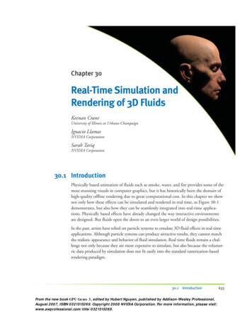
Listing 30-2 (continued). MacCormack Advection SchemenodeValues[4] phi n.Sample(samPointClamp, nposfloat3(ht.x, -ht.y,nodeValues[5] phi n.Sample(samPointClamp, nposfloat3(ht.x, -ht.y,nodeValues[6] phi n.Sample(samPointClamp, nposfloat3(ht.x, ht.y,nodeValues[7] phi n.Sample(samPointClamp, nposfloat3(ht.x, ht.y, -ht.z)); ht.z)); -ht.z)); ht.z));// Determine a valid range for the result.float4 phiMin min(min(min(min(min(min(min(nodeValues[0], nodeValues [1]), nodeValues [2]), nodeValues [3]),nodeValues[4]), nodeValues [5]), nodeValues [6]), nodeValues [7]);float4 phiMax max(max(max(max(max(max(max(nodeValues[0], nodeValues [1]), nodeValues [2]), nodeValues [3]),nodeValues[4]), nodeValues [5]), nodeValues [6]), nodeValues [7]);// Perform final advection, combining values from intermediate// advection steps.float4 r phi n 1 hat.Sample(samLinear, nposTC) 0.5 * (phi n.Sample(samPointClamp, in.CENTERCELL) phi n hat.Sample(samPointClamp, in.CENTERCELL));// Clamp result to the desired range.r max(min(r, phiMax), phiMin);return r;}On the GPU, higher-order schemes are often a better way to get improved visual detailthan simply increasing the grid resolution, because math is cheap compared to bandwidth. Figure 30-3 compares a higher-order scheme on a low-resolution grid with alower-order scheme on a high-resolution grid.30.2.4 Solid-Fluid InteractionOne of the benefits of using real-time simulation (versus precomputed animation) isthat fluid can interact with the environment. Figure 30-4 shows an example on onesuch scene. In this section we discuss two simple ways to allow the environment to acton the fluid.642Chapter 30Real-Time Simulation and Rendering of 3D FluidsCopyright NVIDIA Corporation. All rights reserved.
Figure 30-3. Bigger Is Not Always Better!Left: MacCormack advection scheme (applied to both velocity and smoke density) on a 128 64 64grid. Right: Semi-Lagrangian advection scheme on a 256 128 128 grid.A basic way to influence the velocity field is through the application of external forces.To get the gross effect of an obstacle pushing fluid around, we can approximate theobstacle with a basic shape such as a box or a ball and add the obstacle’s average velocityto that region of the velocity field. Simple shapes like these can be described with animplicit equation of the form f (x, y, z) 0 that can be easily evaluated by a pixel shaderat each grid cell.Although we could explicitly add velocity to approximate simple motion, there aresituations in which more detail is required. In Hellgate: London, for example, wewanted smoke to seep out through cracks in the ground. Adding a simple upward velocity and smoke density in the shape of a crack resulted in uninteresting motion. Instead, we used the crack shape, shown inset in Figure 30-5, to define solid obstacles forsmoke to collide and interact with. Similarly, we wanted to achieve more-precise interactions between smoke and an animated gargoyle, as shown in Figure 30-4. To do so,we needed to be able to affect the fluid motion with dynamic obstacles (see the detailslater in this section), which required a volumetric representation of the obstacle’s interior and of the velocity at its boundary (which we also explain later in this section).Figure 30-4. An Animated Gargoyle Pushes Smoke Around by Flapping Its Wings30.2Copyright NVIDIA Corporation. All rights reserved.Simulation643
Figure 30-5. Smoke Rises from a Crack in the Ground in the Game Hellgate: LondonInset: A slice from the obstacle texture that was used to block the smoke; white texels indicate anobstacle, and black texels indicate open space.Dynamic ObstaclesSo far we have assumed that a fluid occupies the entire rectilinear region defined by thesimulation grid. However, in most applications, the fluid domain (that is, the region ofthe grid actually occupied by fluid) is much more interesting. Various methods forhandling static boundaries on the GPU are discussed in Harris et al. 2003,Liu et al. 2004, Wu et al. 2004, and Li et al. 2005.The fluid domain may change over time to adapt to dynamic obstacles in the environment, and in the case of liquids, such as water, the domain is constantly changing as theliquid sloshes around (more in Section 30.2.7). In this section we describe the schemeused for handling dynamic obstacles in Hellgate: London. For further discussion of dynamic obstacles, see Bridson et al. 2006 and Foster and Fedkiw 2001.To deal with complex domains, we must consider the fluid’s behavior at the domainboundary. In our discretized fluid, the domain boundary consists of the faces betweencells that contain fluid and cells that do not—that is, the face between a fluid cell and asolid cell is part of the boundary, but the solid cell itself is not. A simple example of adomain boundary is a static barrier placed around the perimeter of the simulation gridto prevent fluid from “escaping” (without it, the fluid appears as though it is simplyflowing out into space).644Chapter 30Real-Time Simulation and Rendering of 3D FluidsCopyright NVIDIA Corporation. All rights reserved.
To support domain boundaries that change due to the presence of dynamic obstacles,we need to modify some of our simulation steps. In our implementation, obstacles arerepresented using an inside-outside voxelization. In addition, we keep a voxelized representation of the obstacle’s velocity in solid cells adjacent to the domain boundary. Thisinformation is stored in a pair of 3D textures that are updated whenever an obstaclemoves or deforms (we cover this later in this section).At solid-fluid boundaries, we want to impose a free-slip boundary condition, which saysthat the velocities of the fluid and the solid are the same in the direction normal to theboundary:u n u solid n.In other words, the fluid cannot flow into or out of a solid, but it is allowed to flowfreely along its surface.The free-slip boundary condition also affects the way we solve for pressure, because thegradient of pressure is used in determining the final velocity. A detailed discussion ofpressure projection can be found in Bridson et al. 2006, but ultimately we just need tomake sure that the pressure values we compute satisfy the following: Δt Fpp n di , j ,k ,i , j ,ki , j ,kρΔx 2 n Fi , j ,k where Δt is the size of the time step, Δx is the cell spacing, pi,j,k is the pressure value incell (i, j, k), di,j,k is the discrete velocity divergence computed for that cell, and Fi,j,k isthe set of indices of cells adjacent to cell (i, j, k) that contain fluid. (This equation issimply a discrete form of the pressure-Poisson system 2p w in Harris 2004 thatrespects solid boundaries.) It is also important that at solid-fluid boundaries, di,j,k iscomputed using obstacle velocities.In practice there’s a very simple trick for making sure all this happens: any time wesample pressure from a neighboring cell (for example, in the pressure solve and pressureprojection steps), we check whether the neighbor contains a solid obstacle, as shown inFigure 30-6. If it does, we use the pressure value from the center cell in place of theneighbor’s pressure value. In other words, we nullify the solid cell’s contribution to thepreceding equation.We can apply a similar trick for velocity values: whenever we sample a neighboring cell(for example, when computing the velocity’s divergence), we first check to see if it contains a solid. If so, we look up the obstacle’s velocity from our voxelization and use it inplace of the value stored in the fluid’s velocity field.30.2Copyright NVIDIA Corporation. All rights reserved.Simulation645
-12-14-1SolidFluid-1-1-1Figure 30-6. Accounting for Obstacles in the Computation of the Discrete Laplacian of PressureLeft: A stencil used to compute the discrete Laplacian of pressure in 2D. Right: This stencil changesnear solid-fluid boundaries. Checking for solid neighbors and replacing their pressure values withthe central pressure value results in the same behavior.Because we cannot always solve the pressure-Poisson system to convergence, we explicitly enforce the free-slip boundary condition immediately following pressure projection.We must also correct the result of the pressure projection step for fluid cells next to thedomain boundary. To do so, we compute the obstacle’s velocity component in the direction normal to the boundary. This value replaces the corresponding component ofour fluid velocity at the center cell, as shown in Figure 30-7. Because solid-fluid boundaries are aligned with voxel faces, computing the projection of the velocity onto thesurface normal is simply a matter of selecting the appropriate component.If two opposing faces of a fluid cell are solid-fluid boundaries, we could average thevelocity values from both sides. However, simply selecting one of the two faces generally gives acceptable results.vvu(Before)u(After)Figure 30-7. Enforcing the Free-Slip Boundary Condition After Pressure ProjectionTo enforce free-slip behavior at the boundary between a fluid cell (red) and a solid cell (black), wemodify the velocity of the fluid cell in the normal (u) direction so that it equals the obstacle’svelocity in the normal direction. We retain the fluid velocity in the tangential (v) direction.646Chapter 30Real-Time Simulation and Rendering of 3D FluidsCopyright NVIDIA Corporation. All rights reserved.
Finally, it is important to realize that when very large time steps are used, quantities can“leak” through boundaries during advection. For this reason we add an additional constraint to the advection steps to ensure that we never advect any quantity into the interior of an obstacle, guaranteeing that the value of advected quantities (for example,smoke density) is always zero inside solid obstacles (see the PS ADVECT OBSTACLEroutine in Listing 30-3). In Listing 30-3, we show the simulation kernels modified totake boundary conditions into account.Listing 30-3. Modified Simulation Kernels to Account for Boundary Conditionsbool IsSolidCell(float3 cellTexCoords){return obstacles.Sample(samPointClamp, cellTexCoords).r 0.9;}float PS JACOBI OBSTACLE(GS OUTPUT FLUIDSIM in,Texture3D pressure,Texture3D divergence) : SV Target{// Get the divergence and pressure at the current cell.float dC divergence.Sample(samPointClamp, in.CENTERCELL);float pC pressure.Sample(samPointClamp, in.CENTERCELL);// Get thefloat pL float pR float pB float pT float pD float pU pressure values from neighboring cells.pressure.Sample(samPointClamp, in.LEFTCELL);pressure.Sample(samPointClamp, in.RIGHTCELL);pressure.Sample(samPointClamp, in.BOTTOMCELL);pressure.Sample(samPointClamp, in.TOPCELL);pressure.Sample(samPointClamp, in.DOWNCELL);pressure.Sample(samPointClamp, in.UPCELL);// Make sure that the pressure in solid cells is effectively ignored.if(IsSolidCell(in.LEFTCELL)) pL pC;if(IsSolidCell(in.RIGHTCELL)) pR pC;if(IsSolidCell(in.BOTTOMCELL)) pB pC;if(IsSolidCell(in.TOPCELL)) pT pC;if(IsSolidCell(in.DOWNCELL)) pD pC;if(IsSolidCell(in.UPCELL)) pU pC;// Compute the new pressure value.return(pL pR pB pT pU pD - dC) /6.0;}30.2Copyright NVIDIA Corporation. All rights reserved.Simulation647
Listing 30-3 (continued). Modified Simulation Kernels to Account for Boundary Conditionsfloat4 GetObstacleVelocity(float3 cellTexCoords){return obstaclevelocity.Sample(samPointClamp, cellTexCoords);}float PS DIVERGENCE OBSTACLE(GS OUTPUT FLUIDSIM in,Texture3D velocity) : SV Target{// Get velocity values from neighboring cells.float4 fieldL velocity.Sample(samPointClamp, in.LEFTCELL);float4 fieldR velocity.Sample(samPointClamp, in.RIGHTCELL);float4 fieldB velocity.Sample(samPointClamp, in.BOTTOMCELL);float4 fieldT velocity.Sample(samPointClamp, in.TOPCELL);float4 fieldD velocity.Sample(samPointClamp, in.DOWNCELL);float4 fieldU velocity.Sample(samPointClamp, in.UPCELL);// Use obstacle velocities for any solid cells.if(IsBoundaryCell(in.LEFTCELL))fieldL (in.RIGHTCELL))fieldR l(in.BOTTOMCELL))fieldB ll(in.TOPCELL))fieldT in.DOWNCELL))fieldD (in.UPCELL))fieldU GetObstacleVelocity(in.UPCELL);// Compute the velocity’s divergence using central differences.float divergence 0.5 * ((fieldR.x - fieldL.x) (fieldT.y - fieldB.y) (fieldU.z - fieldD.z));return divergence;}648Chapter 30Real-Time Simulation and Rendering of 3D FluidsCopyright NVIDIA Corporation. All rights reserved.
Listing 30-3 (continued). Modified Simulation Kernels to Account for Boundary Conditionsfloat4 PS PROJECT OBSTACLE(GS OUTPUT FLUIDSIM in,Texture3D pressure,Texture3D velocity): SV Target{// If the cell is solid, simply use the corresponding// obstacle velocity.if(IsBoundaryCell(in.CENTERCELL)){return GetObstacleVelocity(in.CENTERCELL);}// Get pressure values for the current cell and its neighbors.float pC pressure.Sample(samPointClamp, in.CENTERCELL);float pL pressure.Sample(samPointClamp, in.LEFTCELL);float pR pressure.Sample(samPointClamp, in.RIGHTCELL);float pB pressure.Sample(samPointClamp, in.BOTTOMCELL);float pT pressure.Sample(samPointClamp, in.TOPCELL);float pD pressure.Sample(samPointClamp, in.DOWNCELL);float pU pressure.Sample(samPointClamp, in.UPCELL);// Get obstacle velocities in neighboring solid cells.// (Note that these values are meaningless if a neighbor// is not solid.)float3 vL GetObstacleVelocity(in.LEFTCELL);float3 vR GetObstacleVelocity(in.RIGHTCELL);float3 vB GetObstacleVelocity(in.BOTTOMCELL);float3 vT GetObstacleVelocity(in.TOPCELL);float3 vD GetObstacleVelocity(in.DOWNCELL);float3 vU GetObstacleVelocity(in.UPCELL);float3 obstV float3(0,0,0);float3 vMask float3(1,1,1);// If an adjacent cell is solid, ignore its pressure// and use its velocity.if(IsBoundaryCell(in.LEFTCELL)) {pL pC; obstV.x vL.x; vMask.x 0; }if(IsBoundaryCell(in.RIGHTCELL)) {pR pC; obstV.x vR.x; vMask.x 0; }30.2Copyright NVIDIA Corporation. All rights reserved.Simulation649
Listing 30-3 (continued). Modified Simulation Kernels to Account for Boundary Conditionsif(IsBoundaryCell(in.BOTTOMCELL)) {pB pC; obstV.y vB.y; vMask.y if(IsBoundaryCell(in.TOPCELL)) {pT pC; obstV.y vT.y; vMask.y if(IsBoundaryCell(in.DOWNCELL)) {pD pC; obstV.z vD.z; vMask.z if(IsBoundaryCell(in.UPCELL)) {pU pC; obstV.z vU.z; vMask.z 0; }0; }0; }0; }// Compute the gradient of pressure at the current cell by// taking central differences of neighboring pressure values.float gradP 0.5*float3(pR - pL, pT - pB, pU - pD);// Project the velocity onto its divergence-free component by// subtracting the gradient of pressure.float3 vOld velocity.Sample(samPointClamp, in.texcoords);float3 vNew vOld - gradP;// Explicitly enforce the free-s
the realistic appearance and behavior of fluid simulation. Real time fluids remain a chal-lenge not only because they are more expensive to simulate, but also because the volumet-ric data produced by simulation does not fit easily into the standard rasterization-based rendering paradigm. Real-Time Simulation