Transcription
Harmonics Chapter 1, IntroductionApril 2012Understanding Power System HarmonicsProf. Mack GradyDept. of Electrical & Computer EngineeringUniversity of Texas at Austinmack@ieee.org, www.ece.utexas.edu/ gradyTable of Contents Chapter 1. Introduction Chapter 2. Fourier Series Chapter 3. Definitions Chapter 4. Sources Chapter 5. Effects and Symptoms Chapter 6. Conducting an Investigation Chapter 7. Standards and Solutions Chapter 8. System Matrices and Simulation Procedures Chapter 9. Case Studies Chapter 10. Homework Problems Chapter 11. Acknowledgements Appendix A1. Fourier Spectra Data Appendix A2. PCFLO User Manual Appendix A3. Harmonics Analysis for Industrial Power Systems (HAPS) User Manualand Files1.IntroductionPower systems are designed to operate at frequencies of 50 or 60Hz. However, certain types ofloads produce currents and voltages with frequencies that are integer multiples of the 50 or 60 Hzfundamental frequency. These higher frequencies are a form of electrical pollution known aspower system harmonics.Power system harmonics are not a new phenomenon. In fact, a text published by Steinmetz in1916 devotes considerable attention to the study of harmonics in three-phase power systems. InSteinmetz’s day, the main concern was third harmonic currents caused by saturated iron intransformers and machines. He was the first to propose delta connections for blocking thirdharmonic currents.After Steinmetz’s important discovery, and as improvements were made in transformer andmachine design, the harmonics problem was largely solved until the 1930s and 40s. Then, withthe advent of rural electrification and telephones, power and telephone circuits were placed oncommon rights-of-way. Transformers and rectifiers in power systems produced harmoniccurrents that inductively coupled into adjacent open-wire telephone circuits and producedaudible telephone interference. These problems were gradually alleviated by filtering and byMack Grady, Page 1-1
Harmonics Chapter 1, IntroductionApril 2012minimizing transformer core magnetizing currents. Isolated telephone interference problems stilloccur, but these problems are infrequent because open-wire telephone circuits have beenreplaced with twisted pair, buried cables, and fiber optics.Today, the most common sources of harmonics are power electronic loads such as adjustablespeed drives (ASDs) and switching power supplies. Electronic loads use diodes, siliconcontrolled rectifiers (SCRs), power transistors, and other electronic switches to either chopwaveforms to control power, or to convert 50/60Hz AC to DC. In the case of ASDs, DC is thenconverted to variable-frequency AC to control motor speed. Example uses of ASDs includechillers and pumps.A single-phase power electronic load that you are familiar with is the single-phase light dimmershown in Figure 1.1. By adjusting the potentiometer, the current and power to the light bulb arecontrolled, as shown in Figures 1.2 and 1.3.aLightbulbbTriac(front view)3.3kΩMT2 120Vrms AC–250kΩlinearpotcTriacGMT10.1µFBilateral triggerdiode (diac)MT1 MT2 Gna Van– nLightbulb 0V –ab Van–Before firing, the triac is an open switch,so that practically no voltage is appliedacross the light bulb. The small currentthrough the 3.3kΩ resistor is ignored inthis diagram. Van– nLightbulb Van –b 0V–After firing, the triac is a closedswitch, so that practically all of Vanis applied across the light bulb.Figure 1.1. Triac light dimmer circuitMack Grady, Page 1-2
Harmonics Chapter 1, IntroductionApril 2012α 90ºCurrent30 60 90 120 150 180 210 240 270 300 330 3600306090 120 150 180 210 240 270 300 330 360AngleAngleα leFigure 1.2. Light dimmer current waveforms for firing anglesα 30º, 90º, and 150º10.90.80.70.6PCurrentα 30º0.50.40.30.20.100306090120150AlphaFigure 1.3. Normalized power delivered to light bulb versus αMack Grady, Page 1-3180
Harmonics Chapter 1, IntroductionApril 2012The light dimmer is a simple example, but it represents two major benefits of power electronicloads controllability and efficiency. The “tradeoff” is that power electronic loads drawnonsinusoidal currents from AC power systems, and these currents react with system impedancesto create voltage harmonics and, in some cases, resonance. Studies show that harmonicdistortion levels in distribution feeders are rising as power electronic loads continue to proliferateand as shunt capacitors are employed in greater numbers to improve power factor closer to unity.Unlike transient events such as lightning that last for a few microseconds, or voltage sags thatlast from a few milliseconds to several cycles, harmonics are steady-state, periodic phenomenathat produce continuous distortion of voltage and current waveforms. These periodicnonsinusoidal waveforms are described in terms of their harmonics, whose magnitudes andphase angles are computed using Fourier analysis.Fourier analysis permits a periodic distorted waveform to be decomposed into a series containingdc, fundamental frequency (e.g. 60Hz), second harmonic (e.g. 120Hz), third harmonic (e.g.180Hz), and so on. The individual harmonics add to reproduce the original waveform. Thehighest harmonic of interest in power systems is usually the 25th (1500Hz), which is in the lowaudible range. Because of their relatively low frequencies, harmonics should not be confusedwith radio-frequency interference (RFI) or electromagnetic interference (EMI).Ordinarily, the DC term is not present in power systems because most loads do not produce DCand because transformers block the flow of DC. Even-ordered harmonics are generally muchsmaller than odd-ordered harmonics because most electronic loads have the property of halfwave symmetry, and half-wave symmetric waveforms have no even-ordered harmonics.The current drawn by electronic loads can be made distortion-free (i.e., perfectly sinusoidal), butthe cost of doing this is significant and is the subject of ongoing debate between equipmentmanufacturers and electric utility companies in standard-making activities. Two main concernsare1. What are the acceptable levels of current distortion?2. Should harmonics be controlled at the source, or within the power system?Mack Grady, Page 1-4
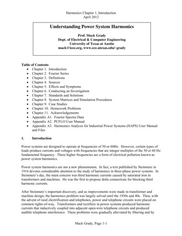
Harmonics Chapter 2, Fourier SeriesApril 20122.Fourier Series2.1.General DiscussionAny physically realizable periodic waveform can be decomposed into a Fourier series of DC,fundamental frequency, and harmonic terms. In sine form, the Fourier series isi (t ) I avg I k sin(k 1t k ) ,(2.1)k 1and if converted to cosine form, 2.1 becomesi (t ) I avg I k cos(k 1t k 90 o ) .k 1I avg is the average (often referred to as the “DC” value I dc ). I k are peak magnitudes of theindividual harmonics, o is the fundamental frequency (in radians per second), and k are theharmonic phase angles. The time period of the waveform isT 2 1 2 1 .2 f1 f1The formulas for computing I dc , I k , k are well known and can be found in any undergraduateelectrical engineering textbook on circuit analysis. These are described in Section 2.2.Figure 2.1 shows a desktop computer (i.e., PC) current waveform. The corresponding spectrumis given in the Appendix. The figure illustrates how the actual waveform can be approximatedby summing only the fundamental, 3rd, and 5th harmonic components. If higher-order terms areincluded (i.e., 7th, 9th, 11th, and so on), then the PC current waveform will be perfectlyreconstructed. A truncated Fourier series is actually a least-squared error curve fit. As higherfrequency terms are added, the error is reduced.Fortunately, a special property known as half-wave symmetry exists for most power electronicloads. Have-wave symmetry exists when the positive and negative halves of a waveform areidentical but opposite, i.e.,i (t ) i (t T),2where T is the period. Waveforms with half-wave symmetry have no even-ordered harmonics.It is obvious that the television current waveform is half-wave symmetric.Mack Grady, Page 2-1
Harmonics Chapter 2, Fourier SeriesApril 2012Amperes50-55AmperesSum of 1st, 3rd, 5th5301-5Figure 2.1. PC Current Waveform, and its 1st, 3rd, and 5th Harmonic Components(Note – in this waveform, the harmonics are peaking at the same time as thefundamental. Most waveforms do not have this property. In fact, in many cases (e.g.a square wave), the peak of the fundamental component is actually greater than thepeak of the composite wave.)Mack Grady, Page 2-2
Harmonics Chapter 2, Fourier SeriesApril 20122.2Fourier CoefficientsIf function i (t ) is periodic with an identifiable period T (i.e., i (t ) i (t NT ) ), then i (t ) can bewritten in rectangular form asi (t ) I avg ak cos(k 1t ) bk sin(k 1t ) , 1 k 12 ,T(2.2)whereI avg 1 t o Ti (t )dt ,T t oak 2 to Ti (t ) cos k 1t dt ,T t obk 2 to Ti (t ) sin k 1t dt .T t oThe sine and cosine terms in (2.2) can be converted to the convenient polar form of (2.1) byusing trigonometry as follows:a k cos(k 1t ) bk sin(k 1t )a cos(k 1t ) bk sin( k 1t ) a k2 bk2 ka k2 bk2 a k2 bk2 bkak cos(k 1t ) sin(k 1t ) 2 222a k bk a k bk a k2 bk2 sin( k ) cos(k 1t ) cos( k ) sin( k 1t ) ,(2.3)wheresin( k ) ak, cos( k ) 22a k bkbka k2 bk2.akApplying trigonometric identitysin( A B) sin( A) cos( B) cos( A) sin( B)Mack Grady, Page 2-3θkbk
Harmonics Chapter 2, Fourier SeriesApril 2012yields polar forma k2 bk2 sin( k 1t k ) ,(2.4)wheretan( k ) 2.3sin( k ) a k. cos( k ) bk(2.5)Phase ShiftThere are two types of phase shifts pertinent to harmonics. The first is a shift in time, e.g. the T/3 among balanced a-b-c currents. If the PC waveform in Figure 2.2 is delayed by Tseconds, the modified current is5Amperesdelayed0-5Figure 2.2. PC Current Waveform Delayed in Timei (t T ) I k sin(k 1 t T k ) k 1 I k sin(k 1t k 1 T k )k 1 I k sin k 1t k k 1 T I k sin k 1t k k 1 ,k 1(2.6)k 1where 1 is the phase lag of the fundamental current corresponding to T . The last term in(2.6) shows that the individual harmonic phase angles are delayed by k 1 of their own degrees.The second type of phase shift is in phase angle, which occurs in wye-delta transformers. Wyedelta transformers shift voltages and currents by 30 o , depending on phase sequence. ANSIstandards require that, regardless of which side is delta or wye, the a-b-c phases must be markedso that the high-voltage side voltages and currents lead those on the low-voltage side by 30 o forMack Grady, Page 2-4
Harmonics Chapter 2, Fourier SeriesApril 2012positive-sequence (and thus lag by 30 o for negative sequence). Zero sequences are blocked bythe three-wire connection so that their phase shift is not meaningful.2.4Symmetry SimplificationsWaveform symmetry greatly simplifies the integration effort required to develop Fouriercoefficients. Symmetry arguments should be applied to the waveform after the average (i.e.,DC) value has been removed. The most important cases are Odd Symmetry, i.e., i (t ) i ( t ) ,then the corresponding Fourier series has no cosine terms,ak 0 ,and bk can be found by integrating over the first half-period and doubling the results,bk 4 T /2i (t ) sin k 1t dt .T 0Even Symmetry, i.e., i (t ) i ( t ) ,then the corresponding Fourier series has no sine terms,bk 0 ,and a k can be found by integrating over the first half-period and doubling the results,ak 4 T /2i (t ) cos k 1t dt .T 0Important note – even and odd symmetry can sometimes be obtained by time-shifting thewaveform. In this case, solve for the Fourier coefficients of the time-shifted waveform, andthen phase-shift the Fourier coefficient angles according to (A.6). Half-Wave Symmetry, i.e., i (t T) i (t ) ,2then the corresponding Fourier series has no even harmonics, and a k and bk can befound by integrating over any half-period and doubling the results,ak 4 to T / 2i (t ) cos k 1t dt ,T t ok odd,Mack Grady, Page 2-5
Harmonics Chapter 2, Fourier SeriesApril 2012bk 4 to T / 2i (t ) sin k 1t dt ,T t ok odd.Half-wave symmetry is common in power systems.2.5Examples T/2Square WaveVBy inspection, the average value is zero, andthe waveform has both odd symmetry andhalf-wave symmetry. Thus, a k 0 , andbk –V4 to T / 2v(t ) sin k 1t dt , k odd.T t oTSolving for bk ,bk 4V 4V4 T /2t T / 2cos k 1t t 0 V sin k 1t dt 0Tk oTk 1TSince 1 k 1T cos cos(0) . 2 2 , thenTbk 4V cos k 1 2V 1 cos k , yieldingk 2k bk 4V, k odd.k The Fourier series is thenv(t ) 14V 11 sin k 1t sin 1 1t sin 3 1t sin 5 1t . (2.7) k 1, k odd k 35 4V Note that the harmonic magnitudes decrease according toMack Grady, Page 2-61.k
Harmonics Chapter 2, Fourier SeriesApril 2012 T/2Triangle WaveVBy inspection, the average value is zero, andthe waveform has both even symmetry andhalf-wave symmetry. Thus, bk 0 , andak –V4 to T / 2v(t ) cos k 1t dt , k odd.T t oTSolving for a k ,ak 4 T / 2 4t 4V T / 216V T / 2cos k 1t dt V 1 cos k 1t dt t cos k 1t dtT 0T 0 T T2 04V k 1Tt T / 2 k 1T 16V t sin k 1t sin sin(0) 2k 1 2 Tt 0 16V T / 2 sin k 1t dt k 1T2 02V4V4V 1 cos k , k odd.sin k sin k k k k 2 2 Continuing,ak 8Vk 2 2, k odd.The Fourier series is thenv(t ) 8V 2 k 1, k odd1k2cos k 1t 18V 1 cos 1 1t cos 3 1t cos 5 1t ,2 259 where it is seen that the harmonic magnitudes decrease according to(2.8)1k2.To convert to a sine series, recall that cos( ) sin( 90 o ) , so that the series becomesMack Grady, Page 2-7
Harmonics Chapter 2, Fourier SeriesApril 2012 18V 1 sin 1 1t 90 o sin 3 1t 90 o sin 5 1t 90 o .2 259 v(t ) To time delay the waveform by (2.9)T(i.e., move to the right by 90 o of fundamental),4subtract k 90 o from each harmonic angle. Then, (2.9) becomes 8V 1 sin 1 1t 90 o 1 90 o sin 3 1t 90 o 3 90 o 9 2 1 sin 5 1t 90 o 5 90 o ,25 v(t ) orv(t ) 118V 1 sin 1 1t sin 3 1t sin 5 1t sin 7 1t . 2 49259 Half-Wave Rectified Cosine Waveak TIThe waveform has an average value and evensymmetry. Thus, bk 0 , and(2.10)T/24 T /2i (t ) cos k o t dt , k odd.T 0T/2Solving for the average value,t T / 41 t T1 T /4Isin 1t I avg o i (t )dt I cos 1t dt /4tT oTT oTt T / 4 T 1 1T I I 1T sin sin sin 1 sin .2 2 44 4I avg I .(2.11)Solving for a k ,ak 4 T /42II cos 1t cos k 1t dt T 0TT /4 cos 1 k 1t cos 1 k 1t dt0Mack Grady, Page 2-8
Harmonics Chapter 2, Fourier SeriesApril 20122 I sin 1 k 1t sin 1 k 1t 1 k 1 T 1 k 1t T / 4.t 0For k 1 , taking the limits of the above expression when needed yields T sin 1 k 1 2I4 I sin lim a1 1 k 1 2 T (1 k ) 1 0 sin 1 k 1 0 I sin 0 2I.lim 2 T (1 k ) 1 0 1 k 1 a1 (2.12)2I TI 0 0 0 .T 42For k 1 , sin 1 k sin 1 k I 2 2ak 1 k 1 k . (2.13)All odd k terms in (2.13) are zero. For the even terms, it is helpful to find a commondenominator and write (2.13) as 1 k sin 1 k 1 k sin 1 k I22ak 2 1 k , k 1 , k even. Evaluating the above equation shows an alternating sign pattern that can be expressed asak 2I 1 k 2, 4,6, k 2212k 1, k 1 , k even.The final expression becomesi (t ) I2I 1 k / 2 1 21 cos k 1t cos 1t 2 k 2,4,6, k 1IMack Grady, Page 2-9
Harmonics Chapter 2, Fourier SeriesApril 2012 I2I cos 1t 2 I11 1 3 cos 2 1t 15 cos 4 1t 35 cos 6 1t .(2.14)Light Dimmer CurrentThe Fourier coefficients of the current waveform shown in Figure 1.2 can be shown to bethe following:For the fundamental,a1 Ip1 sin 2 ,sin 2 , b1 I p 1 2 (2.15)where firing angle α is in radians, and I p is the peak value of the fundamental currentwhen 0 .For harmonic multiples above the fundamental (i.e., k 3, 5, 7 , ),ak Ip 1 cos(1 k ) cos(1 k ) 1 cos(1 k ) cos(1 k ) , (2.16) 1 k1 k bk Ip 1 sin(1 k ) sin(1 k ) 1 sin(1 k ) sin(1 k ) . 1 k1 k (2.17)The waveform has zero average, and it has no even harmonics because of half-wavesymmetry.The magnitude of any harmonic k , including k 1, is I k a k2 bk2 . Performing thecalculations for the special case of α I1 I3 I1Ip 1 211 24 2radians (i.e., 90 ) yields 0.593 I p , and I 3 Ip 0.318 I p , 0.537.4The above case is illustrated in the following Excel spreadsheet.Mack Grady, Page 2-10
GradyChapter 2. Fourier SeriesJune 2006Page 2-11Light Dimmer Fourier Waveform.xlsNote – in the highlighted cells, the magnitude of I1 is computed to be 0.593 times the peak value of the fundamental current for the 0 case. The ratio of I3 to I1 is computed to be 0.537.Mack Grady, Page 2-11
Harmonics Chapter 3, DefinitionsApril 20123.Definitions3.1.RMSThe squared rms value of a periodic current (or voltage) waveform is defined as1 T2I rmsto T i(t )2dt .(3.1)toIt is clear in (3.1) that the squared rms value of a periodic waveform is the average value of thesquared waveform.If the current is sinusoidal, the rms value is simply the peak value divided bythe waveform has Fourier series2 . However, if I k sin(k 1t k ) ,i (t ) k 1then substituting into (3.1) yieldsto T2 I k sin(k 1t k ) dt T t o k 112 I rms2 I rms2I rmst T 1 o 22 Isin(k t )2I m I n sin( m 1t m ) sin(n 1t n ) dt 1k k Tm 1, n 1,m nto k 1 t T1 o 2 1 cos 2( k 1t k ) I T k 1 k 2 to cos((m n) 1t m n ) cos((m n) 1t m n ) ImIn dt22 m 1, n 1,m n (3.2)Equation (3.2) is complicated, but most of its terms contribute nothing to the rms value if onethinks of (3.2) as being the average value for one fundamental period. The average value of eachcos 2(k 1t k ) term is zero because the average value of a cosine is zero for one or moreinteger periods. Likewise, the average value of each cos((m n) 1t m n ) term is also zerobecause m and n are both harmonics of the fundamental. Thus, (3.2) reduces to2I rmst T21 o 2 1 1 21 2 Ik , IdtItTtI ooT k 1 k 2 2T k 1 k2 k 1 k k 1 2 toMack Grady, Page 3-1(3.3)
Harmonics Chapter 3, DefinitionsApril 2012where I k are peak values of the harmonic components. Factoring out the2I rms I12, rms I 22, rms I 32, rms .2 yields(3.4)Equations (3.3) and (3.4) ignore any DC that may be present. The effect of DC is to add the term2to (3.3) and (3.4).I DCThe cross products of unlike frequencies contribute nothing to the rms value of the totalwaveform. The same statement can be made for average power, as will be shown later.Furthermore, since the contribution of harmonics to rms add in squares, and their magnitudes areoften much smaller than the fundamental, the impact of harmonics on rms is usually not great.3.2.THDThe most commonly-used measure for harmonics is total harmonic distortion (THD), also knownas distortion factor. It is applied to both voltage and current. THD is defined as the rms value ofthe harmonics above fundamental, divided by the rms value of the fundamental. DC is ignored.Thus, for current, THD I I k2 k 2 I122 1 2 I2 k 2 kI1.2The same equation form applies to voltage THDV .THD and rms are directly linked. Note that since2I rms 1 2 I2 k 1 kand sinceTHD I2 1 2 I2 k 2 kI122 2 2 I I1k k 1 ,I12then rewriting yieldsMack Grady, Page 3-2(3.5)
Harmonics Chapter 3, DefinitionsApril 2012 I k2 I12 1 THDI2 , k 1so that 1 2 I12Ik 1 THD I2 . 2 k 12Comparing to (3.3) yields2I rms 1 2 I12 I 2 1 THDI2 I12,rms 1 THDI2 .2 k 1 kThus the equation linking THD and rms isI rms I1, rms 1 THD I2 .(3.6)Because 1. line losses are proportional to the square of rms current (and sometimes increasemore rapidly due to the resistive skin effect), and 2. rms increases with harmonics, then linelosses always increase when harmonics are present. For example, many PCs have a currentdistortion near 1.0 (i.e., 100%). Thus, the wiring losses incurred while supplying a PC are twicewhat they would be in the sinusoidal case.Current distortion in loads varies from a few percent to more than 100%, but voltage distortion isgenerally less than 5%. Voltage THDs below 0.05, i.e. 5%, are considered acceptable, and thosegreater than 10% are definitely unacceptable and will cause problems for sensitive equipmentand loads.3.3.Average PowerHarmonic powers (including the fundamental) add and subtract independently to produce totalaverage power. Average power is defined as1Pavg Tt o T1 p(t )dt Ttoto T v(t )i(t )dt .toSubstituting in the Fourier series of voltage and current yields1Pavg Tto T Vk sin( k 1t k ) I k sin( k 1t k ) dt , k 1 t o k 1Mack Grady, Page 3-3(3.7)
Harmonics Chapter 3, DefinitionsApril 2012and expanding yieldst T1 o Pavg Vk I k sin(k 1t k ) sin(k 1t k )T k 1to , VIsin(m t )sin(n t ) mn11mn dtm 1, n 1,m n t T1 o cos( k k ) cos(2k 1t k k ) Pavg Vk I k 2T t k 1o cos((m n) 1t m n ) cos((m n) 1t m n ) ImIn dt22 m 1, n 1,m n As observed in the rms case, the average value of all the sinusoidal terms is zero, leaving onlythe time invariant terms in the summation, orPavg V Ik k k 1 2cos( k k ) Vk ,rms I k ,rms dpf kk 1 P1,avg P2,avg P3,avg ,(3.8)where dpf k is the displacement power factor for harmonic k .The harmonic power terms P2, avg , P3, avg , are mostly losses and are usually small in relationto total power. However, harmonic losses may be a substantial part of total losses.Equation (3.8) is important in explaining who is responsible for harmonic power. Electric utilitygenerating plants produce sinusoidal terminal voltages. According to (3.8), if there is noharmonic voltage at the terminals of a generator, then the generator produces no harmonicpower. However, due to nonlinear loads, harmonic power does indeed exist in power systemsand causes additional losses. Thus, it is accurate to say that Harmonic power is parasitic and is due to nonlinear equipment and loads. The source of most harmonic power is power electronic loads. By chopping the 60 Hz current waveform and producing harmonic voltages and currents,power electronic loads convert some of the “60 Hz” power into harmonic power, whichin turn propagates back into the power system, increasing system losses and impactingsensitive loads.For a thought provoking question related to harmonic power, consider the case shown in Figure3.1 where a perfect 120Vac(rms) power system with 1Ω internal resistance supplies a triacMack Grady, Page 3-4
Harmonics Chapter 3, DefinitionsApril 2012controlled 1000W incandescent lamp. Let the firing angle is 90 , so the lamp is operating athalf-power.Current i1Ωi vsvm––Customer14.4ΩFigure 3.1. Single-Phase Circuit with Triac and Lamp120 2Assuming that the resistance of the lamp is 14.4Ω, and that the voltage source is1000v s (t ) 120 2 sin( 1t ) , then the Fourier series of current in the circuit, truncated at the 5thharmonic, isi (t ) 6.99 sin( 1t 32.5 o ) 3.75 sin(3 1t 90.0 o ) 1.25 sin(5 1t 90.0 o ) .If a wattmeter is placed immediately to the left of the triac, the metered voltage isv m (t ) v s (t ) iR 120 2 sin( 1t ) 1 6.99 sin( 1t 32.5 o ) 3.75 sin(3 1t 90.0 o ) 1.25 sin(5 1t 90.0 o ) 163.8 sin( 1t 1.3o ) 3.75 sin(3 1t 90.0 o ) 1.25 sin(5 1t 90.0 o )and the average power flowing into the triac-lamp customer is 163.8 6.993.75 3.75cos 1.3o ( 32.5 o ) cos 90.0 o ( 90.0 o )221.25 1.25 cos 90.0 o ( 90.0 o )2Pavg Mack Grady, Page 3-5
Harmonics Chapter 3, DefinitionsApril 2012 475.7 – 7.03 – 0.78 467.9WThe first term, 475.7W, is due to the fundamental component of voltage and current. The 7.03Wand 0.78W terms are due to the 3rd and 5th harmonics, respectively, and flow back into the powersystem.The question now is: should the wattmeter register only the fundamental power, i.e., 475.7W, orshould the wattmeter credit the harmonic power flowing back into the power system and registeronly 475.7 – 7.81 467.9W? Remember that the harmonic power produced by the load isconsumed by the power system resistance.3.4.True Power FactorTo examine the impact of harmonics on power factor, it is important to consider the true powerfactor, which is defined aspf true PavgVrms I rms.(3.9)In sinusoidal situations, (3.9) reduces to the familiar displacement power factorV1 I1cos( 1 1 )P1, avg 2 cos( 1 1 ) .dpf1 V1 I1V1, rms I1, rms2When harmonics are present, (3.9) can be expanded aspf true P1, avg P2, avg P3, avg V1, rms 1 THDV2 I1, rms 1 THD I2.In most instances, the harmonic powers are small compared to the fundamental power, and thevoltage distortion is less than 10%. Thus, the following important simplification is usually valid:pf true P1, avgV1, rms I1, rms 1 THD I2 dpf11 THD I2.(3.10)It is obvious in (3.10) that the true power factor of a nonlinear load is limited by its THD I . Forexample, the true power factor of a PC with THD I 100% can never exceed 0.707, no matterhow good its displacement power is. Some other examples of “maximum” true power factor(i.e., maximum implies that the displacement power factor is unity) are given below in Table 3.1.Mack Grady, Page 3-6
Harmonics Chapter 3, DefinitionsApril 2012Table 3.1. Maximum True Power Factor of a Nonlinear Load.CurrentTHDMaximumpf true0.980.890.7120%50%100%3.5.K FactorLosses in transformers increase when harmonics are present because1. harmonic currents increase the rms current beyond what is needed to provide load power,2. harmonic currents do not flow uniformly throughout the cross sectional area of aconductor and thereby increase its equivalent resistance.Dry-type transformers are especially sensitive to harmonics. The K factor was developed toprovide a convenient measure for rating the capability of transformers, especially dry types, toserve distorting loads without overheating. The K factor formula is k 2 I k2K k 1. (3.11) I k2k 1In most situations, K 10 .3.6.Phase ShiftThere are two types of phase shifts pertinent to harmonics. The first is a shift in time, e.g. the2Tamong the phases of balanced a-b-c currents. To examine time shift, consider Figure 3.2. 3If the PC waveform is delayed by T seconds, the modified current isi (t T ) I k sin(k 1 t T k ) k 1 I k sin(k 1t k 1 T k )k 1 I k sin k 1t k k 1 T I k sin k 1t k k 1 ,k 1(3.12)k 1where 1 is the phase lag of the fundamental current corresponding to T . The last term in(3.12) shows that individual harmonics are delayed by k 1 .Mack Grady, Page 3-7
Harmonics Chapter 3, DefinitionsApril 20125Amperesdelayed0-5Figure 3.2. PC Current Waveform Delayed in TimeThe second type of phase shift is in harmonic angle, which occurs in wye-delta transformers.Wye-delta transformers shift voltages and currents by 30 o . ANSI standards require that,regardless of which side is delta or wye, the a-b-c phases must be marked so that the highvoltage side voltages and currents lead those on the low-voltage side by 30 o for positive-sequence, and lag by 30 o for negative sequence. Zero sequences are blocked by the three-wireconnection so that their phase shift is not meaningful.3.7.Voltage and Current Phasors in a Three-Phase SystemPhasor diagrams for line-to-neutral and line-to-line voltages are shown in Figure 3.3. Phasorcurrents for a delta-connected load, and their relationship to line currents, are shown in Figure3.4.Mack Grady, Page 3-8
Harmonics Chapter 3, DefinitionsApril 2012ImaginaryVcnVca Vcn – VanVab Van – Vbn30 RealVan120 VbnVbc Vbn – VcnFigure 3.3. Voltage Phasors in a Balanced Three-Phase System(The phasors are rotating counter-clockwise. The magnitude of line-to-line voltage phasors isof line-to-neutral voltage phasors.)Mack Grady, Page 3-93 times the magnitude
Harmonics Chapter 3, DefinitionsApril 2012ImaginaryVcnVca Vcn – VanVab Van – VbnIcIca30 IabRealIaIbVanLine currents Ia, Ib, and IcIbcDelta currents Iab, Ibc, and IcaIccVbnIcaBalanced Sets Add to Zero in BothTime and Phasor DomainsIbcI a Ib I c 0Van Vbn Vcn 0Vab Vbc Vca 0Vbc Vbn – VcnIbIabb–aVab IaFigure 3.4. Currents in a Delta-Connected Load1times the magnitude of line currents Ia, Ib, Ic.)(Conservation of power requires that the magnitudes of delta currents Iab, Ica, and Ibc are3Mack Grady, Page 3-10
Harmonics Chapter 3, DefinitionsApril 20123.8.Phase SequenceIn a balanced three-phase power system, the currents in phases a-b-c are shifted in time by 120 o of fundamental. Therefore, sinceia (t ) I k sin(k 1t k ) ,k 1then the currents in phases b and c lag and lead byib (t ) ic (t ) I k sin(k 1t k kk 1 I k sin(k 1t k kk 12 radians, respectively. Thus32 ),32 ).3Picking out the first three harmonics shows an important pattern. Expanding the above series,ia (t ) I1 sin(1 1t 1 ) I 2 sin(2 1t 2 ) I 3 sin(3 1t 3 ) ,ib (t ) I1 sin(1 1t 1 I1 sin(1 1t 1 2 2 ) I 2 sin(2 1t 2 ) I 3 sin(3 1t 3 0) .33ic (t ) I1 sin(1 1t 1 I1 sin(1 1t 1 2 4 6 ) I 2 sin(2 1t 2 ) I 3 sin(3 1t 3 ) , or3332 4 6 ) I 2 sin(2 1t 2 ) I 3 sin(3 1t 3 ) , or3332 2 ) I 2 sin(2 1t 2 ) I 3 sin(3 1t 3 0) .33By examining the current equations, it can be seen that the first harmonic (i.e., the fundamental) is positive sequence (a-b
The current drawn by electronic loads can be made distortion-free (i.e., perfectly sinusoidal), but the cost of doing this is significant and is the subject of ongoing debate between equipment manufacturers and electric utility companies in standard-making activities. Two main concerns are 1. What are the acc