Transcription
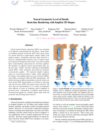
Neural Geometric Level of Detail:Real-time Rendering with Implicit 3D ShapesTowaki Takikawa1,2,4 Joey Litalien1,3 Kangxue Yin1Karsten Kreis1Charles Loop1321,3Derek NowrouzezahraiAlec JacobsonMorgan McGuireSanja Fidler1,2,412NVIDIA3University of TorontoMcGill University4Vector Institutenv-tlabs.github.io/nglodAbstractNeural signed distance functions (SDFs) are emergingas an effective representation for 3D shapes. State-of-theart methods typically encode the SDF with a large, fixedsize neural network to approximate complex shapes withimplicit surfaces. Rendering with these large networks is,however, computationally expensive since it requires manyforward passes through the network for every pixel, makingthese representations impractical for real-time graphics.We introduce an efficient neural representation that, forthe first time, enables real-time rendering of high-fidelityneural SDFs, while achieving state-of-the-art geometryreconstruction quality. We represent implicit surfacesusing an octree-based feature volume which adaptivelyfits shapes with multiple discrete levels of detail (LODs),and enables continuous LOD with SDF interpolation. Wefurther develop an efficient algorithm to directly render ournovel neural SDF representation in real-time by queryingonly the necessary LODs with sparse octree traversal. Weshow that our representation is 2–3 orders of magnitudemore efficient in terms of rendering speed compared toprevious works. Furthermore, it produces state-of-the-artreconstruction quality for complex shapes under both 3Dgeometric and 2D image-space metrics.19.25 KB56.00 KB210.75 KB903.63 KB22.533.54Figure 1: Levels of Detail. Our representation pools features frommultiple scales to adaptively reconstruct high-fidelity geometrywith continuous level of detail (LOD). The subfigures show surfaces (blue) at varying LODs, superimposed on the correspondingcoarse, sparse octrees (orange) which contain the features of thelearned signed distance functions. These were directly rendered inreal-time using our efficient sparse sphere tracing algorithm.1. IntroductionAdvanced geometric modeling and rendering techniquesin computer graphics use 3D shapes with complex details,arbitrary topology, and quality, usually leveraging polygonmeshes. However, it is non-trivial to adapt those representations to learning-based approaches since they lack differentiability, and thus cannot easily be used in computer vision applications such as learned image-based 3D reconstruction. Recently, neural approximations of signed distance functions (neural SDFs) have emerged as an attrac Authors7.63 KBtive choice to scale up computer vision and graphics applications. Prior works [39, 33, 7, 9] have shown that neuralnetworks can encode accurate 3D geometry without restrictions on topology or resolution by learning the SDF, whichdefines a surface by its zero level-set. These works commonly use a large, fixed-size multi-layer perceptron (MLP)as the learned distance function.Directly rendering and probing neural SDFs typically relies on sphere tracing [19], a root-finding algorithm that cancontributed equally.1
Figure 2: We are able to fit shapes of varying complexity, style, scale, with consistently good quality, while being able to leverage thegeometry for shading, ambient occlusion [12], and even shadows with secondary rays. Best viewed zoomed in. We introduce the first real-time rendering approach forcomplex geometry with neural SDFs.require hundreds of SDF evaluations per pixel to converge.As a single forward pass through a large MLP-based SDFcan require millions of operations, neural SDFs quickly become impractical for real-time graphics applications as thecost of computing a single pixel inflates to hundreds of millions of operations. Works such as Davies et al. [9] circumvent this issue by using a small neural network to overfitsingle shapes, but this comes at the cost of generality andreconstruction quality. Previous approaches also use fixedsize neural networks, making them unable to express geometry with complexity exceeding the capacity of the network.In this paper, we present a novel representation for neural SDFs that can adaptively scale to different levels of detail (LODs) and reconstruct highly detailed geometry. Ourmethod can smoothly interpolate between different scalesof geometry (see Figure 1) and can be rendered in real-timewith a reasonable memory footprint. Similar to Davies etal. [9], we also use a small MLP to make sphere tracingpractical, but without sacrificing quality or generality.We take inspiration from classic surface extractionmechanisms [28, 13] which use quadrature and spatial datastructures storing distance values to finely discretize the Euclidean space such that simple, linear basis functions can reconstruct the geometry. In such works, the resolution or treedepth determines the geometric level of detail (LOD) anddifferent LODs can be blended with interpolation. However, they usually require high tree depths to recreate a solution with satisfying quality.In contrast, we discretize the space by using a sparsevoxel octree (SVO) and we store learned feature vectors instead of signed distance values. These vectors can be decoded into scalar distances using a shallow MLP, allowingus to truncate the tree depth while inheriting the advantagesof classic approaches (e.g., LOD). We additionally developa ray traversal algorithm tailored to our architecture, whichallows us to render geometry close to 100 faster thanDeepSDF [39]. Although direct comparisons with neuralvolumetric rendering methods are not possible, we reportframetimes over 500 faster than NeRF [34] and 50 fasterthan NSVF [26] in similar experimental settings.In summary, our contributions are as follows: We propose a neural SDF representation that can efficiently capture multiple LODs, and reconstruct 3Dgeometry with state-of-the-art quality (see Figure 2). We show that our architecture can represent 3D shapesin a compressed format with higher visual fidelity thantraditional methods, and generalizes across differentgeometries even from a single learned example.Due to the real-time nature of our approach, we envision this as a modular building block for many downstream applications, such as scene reconstruction from images, robotics navigation, and shape analysis.2. Related WorkOur work is most related to prior research on mesh simplification for level of detail, 3D neural shape representations, and implicit neural rendering.Level of Detail. Level of Detail (LOD) [29] in computergraphics refers to 3D shapes that are filtered to limit feature variations, usually to approximately twice the pixelsize in image space. This mitigates flickering caused byaliasing, and accelerates rendering by reducing model complexity. While signal processing techniques can filter textures [49], geometry filtering is representation-specific andchallenging. One approach is mesh decimation, where amesh is simplified to a budgeted number of faces, vertices,or edges. Classic methods [15, 20] do this by greedily removing mesh elements with the smallest impact on geometric accuracy. More recent methods optimize for perceptualmetrics [25, 24, 8] or focus on simplifying topology [31].Meshes suffer from discretization errors under low memory constraints and have difficulty blending between LODs.In contrast, SDFs can represent smooth surfaces with lessmemory and smoothly blend between LODs to reduce aliasing. Our neural SDFs inherit these properties.Neural Implicit Surfaces. Implicit surface-based methods encode geometry in latent vectors or neural networkweights, which parameterize surfaces through level-sets.2
Query pointOctree feature volumeVoxel feature retrievalTrilinear eddistanceFigure 3: Architecture. We encode our neural SDF using a sparse voxel octree (SVO) which holds a collection of features Z. The levels ofthe SVO define LODs and the voxel corners contain feature vectors defining local surface segments. Given query point x and LOD L, we(j)find corresponding voxels V1:L , trilinearly interpolate their corners zV up to L and sum to obtain a feature vector z(x). Together with x,bthis feature is fed into a small MLP fθL to obtain a signed distance dL . We jointly optimize MLP parameters θ and features Z end-to-end.3. MethodSeminal works [39, 33, 7] learn these iso-surfaces by encoding the shapes into latent vectors using an auto-decoder—alarge MLP which outputs a scalar value conditional on thelatent vector and position. Another concurrent line of work[47, 45] uses periodic functions resulting in large improvements in reconstruction quality. Davies et al. [9] proposesto overfit neural networks to single shapes, allowing a compact MLP to represent the geometry. Works like CurriculumDeepSDF [11] encode geometry in a progressively growing network, but discard intermediate representations. BSPNet and CvxNet [6, 10] learn implicit geometry with spacepartitioning trees. PIFu [42, 43] learns features on a dense2D grid with depth as an additional input parameter, whileother works learn these on sparse regular [16, 4] or deformed [14] 3D grids. PatchNets [48] learn surface patches,defined by a point cloud of features. Most of these worksrely on an iso-surface extraction algorithm like MarchingCubes [28] to create a dense surface mesh to render the object. In contrast, in this paper we present a method thatdirectly renders the shape at interactive rates.Our goal is to design a representation which reconstructsdetailed geometry and enables continuous level of detail,all whilst being able to render at interactive rates. Figure 3shows a visual overview of our method. Section 3.1 provides a background on neural SDFs and its limitations. Wethen present our method which encodes the neural SDF in asparse voxel octree in Section 3.2 and provide training details in Section 3.3. Our rendering algorithm tailored to ourrepresentation is described in Section 3.4.3.1. Neural Signed Distance Functions (SDFs)SDFs are functions f : R3 R where d f (x)is the shortest signed distance from a point x to a surfaceS M of a volume M R3 , where the sign indicateswhether x is inside or outside of M. As such, S is implicitlyrepresented as the zero level-set of f : (1)S x R3 f (x) 0 .A neural SDF encodes the SDF as the parameters θ of a neural network fθ .–Retrieving the signed distance for apoint x R3 amounts to computingb The parameters θ are optimized with thefθ (x) d. loss J(θ) Ex,d L fθ (x), d , where d is the ground-truthsigned distance and L is some distance metric such as L2 distance. An optional input “shape” feature vector z Rmcan be used to condition the network to fit different shapeswith a fixed θ.To render neural SDFs directly, ray-tracing can be donewith a root-finding algorithm such as sphere tracing [19].This algorithm can perform up to a hundred distance queriesper ray, making standard neural SDFs prohibitively expensive if the network is large and the distance query is tooslow. Using small networks can speed up this iterative rendering process, but the reconstructed shape may be inaccurate. Moreover, fixed-size networks are unable to fit highlycomplex shapes and cannot adapt to simple or far-away objects where visual details are unnecessary.In the next section, we describe a framework that addresses these issues by encoding the SDF using a sparseNeural Rendering for Implicit Surfaces. Many works focus on rendering neural implicit representations. Niemeyeret al. [36] proposes a differentiable renderer for implicit surfaces using ray marching. DIST [27] and SDFDiff [22]present differentiable renderers for SDFs using sphere tracing. These differentiable renderers are agnostic to the raytracing algorithm; they only require the differentiabilitywith respect to the ray-surface intersection. As such, wecan leverage the same techniques proposed in these worksto make our renderer also differentiable. NeRF [34] learnsgeometry as density fields and uses ray marching to visualize them. IDR [50] attaches an MLP-based shading function to a neural SDF, disentangling geometry and shading.NSVF [26] is similar to our work in the sense that it also encodes feature representations with a sparse octree. In contrast to NSVF, our work enables level of detail and usessphere tracing, which allows us to separate out the geometryfrom shading and therefore optimize ray tracing, somethingnot possible in a volumetric rendering framework. As mentioned previously, our renderer is two orders of magnitudefaster compared to numbers reported in NSVF [26].3
where L ⌊L̃⌋ and α L̃ ⌊L̃⌋ is the fractional part,allowing us to smoothly transition between LODs (see Figure 1). This simple blending scheme only works for SDFs,and does not work well for density or occupancy and is illdefined for meshes and point clouds. We discuss how weset the continuous LOD L̃ at render-time in Section 3.4.voxel octree, allowing the representation to adapt to different levels of detail and to use shallow neural networks toencode geometry whilst maintaining geometric accuracy.3.2. Neural Geometric Levels of DetailFramework. Similar to standard neural SDFs, we represent SDFs using parameters of a neural network and an additional learned input feature which encodes the shape. Instead of encoding shapes using a single feature vector z asin DeepSDF [39], we use a feature volume which containsa collection of feature vectors, which we denote by Z.We store Z in a sparse voxel octree (SVO) spanning thebounding volume B [ 1, 1]3 . Each voxel V in the SVO(j)holds a learnable feature vector zV Z at each of its eightcorners (indexed by j), which are shared if neighbour voxelsexist. Voxels are allocated only if the voxel V contains asurface, making the SVO sparse.Each level L N of the SVO defines a LOD for the geometry. As the tree depth L in the SVO increases, the surface is represented with finer discretization, allowing reconstruction quality to scale with memory usage. We denotethe maximum tree depth as Lmax . We additionally employsmall MLP neural networks fθ1:Lmax , denoted as decoders,with parameters θ1:Lmax {θ1 , . . . , θLmax } for each LOD.To compute an SDF for a query point x R3 at thedesired LOD L, we traverse the tree up to level L to findall voxels V1:L {V1 , . . . , VL } containing x. For eachlevel ℓ {1, . . . , L}, we compute a per-voxel shape vector ψ(x; ℓ, Z) by trilinearly interpolating the corner featuresof the voxels at x. WePLsum the features across the levelsto get z(x; L, Z) ℓ 1 ψ(x; ℓ, Z), and pass them intothe MLP with LOD-specific parameters θL . Concretely, wecompute the SDF as dbL fθL [x , z(x; L, Z)] ,(2)3.3. TrainingWe ensure that each discrete level L of the SVO represents valid geometry by jointly training each LOD. We doso by computing individual losses at each level and summing them across levels:J(θ, Z) Ex,dL 1 fθL [x , z(x; L, Z)] d2.(4)We then stochastically optimize the loss function with respect to both θ1:Lmax and Z. The expectation is estimatedwith importance sampling for the points x B. We usesamples from a mixture of three distributions: uniform samples in B, surface samples, and perturbed surface samples.We detail these sampling algorithms and specific traininghyperparameters in the supplementary materials.3.4. Interactive RenderingSphere Tracing. We use sphere tracing [19] to render ourrepresentation directly. Rendering an SVO-based SDF using sphere tracing, however, raises some technical implications that need to be addressed. Typical SDFs are definedon all of R3 . In contrast, our SVO SDFs are defined only forvoxels V which intersect the surface geometry. Therefore,proper handling of distance queries made in empty space isrequired. One option is to use a constant step size, i.e. raymarching, but there is no guarantee the trace will convergebecause the step can overshoot.Instead, at the beginning of the frame we first perform aray-SVO intersection (details below) to retrieve every voxelV at each resolution ℓ that intersects with the ray. Formally,if r(t) x0 td, t 0 is a ray with origin x0 R3 anddirection d R3 , we let Vℓ (r) denote the depth-ordered setof intersected voxels by r at level ℓ.Each voxel in Vℓ (r) contains the intersected ray index,voxel position, parent voxel, and pointers to the eight corner(j)feature vectors zV . We retrieve pointers instead of featurevectors to save memory. The feature vectors are stored ina flatenned array, and the pointers are precalculated in aninitialization step by iterating over all voxels and findingcorresponding indices to the features in each corner.where [ · , · ] denotes concatenation. This summation acrossLODs allows meaningful gradients to propagate acrossLODs, helping especially coarser LODs.(j)Since our shape vectors zV now only represent smallsurface segments instead of entire shapes, we can move thecomputational complexity out of the neural network fθ andinto the feature vector query ψ : R3 Rm , which amountsto a SVO traversal and a trilinear interpolation of the voxelfeatures. This key design decision allows us to use verysmall MLPs, enabling significant speed-ups without sacrificing reconstruction quality.Level Blending. Although the levels of the octree are discrete, we are able to smoothly interpolate between them. Toobtain a desired continuous LOD L̃ 1, we blend betweendifferent discrete octree LODs L by linearly interpolatingthe corresponding predicted distances:dbL̃ (1 α) dbL α dbL 1 ,LmaxXAdaptive Ray Stepping. For a given ray in a spheretrace iteration k, we perform a ray-AABB intersection [30]against the voxels in the target LOD level L to retrieve thefirst voxel VL VL (r) that hits. If xk / VL , we advance xto the ray-AABB intersection point. If xk VL , we query(3)4
No hiteach iteration, we determine the ray-voxel pairs that resultin intersections in D ECIDE, which returns a list of decisionsD with Dj 1 if the ray intersects the voxel and Dj 0otherwise (line 4). Then, we use E XCLUSIVE S UM to compute the exclusive sum S of list D, which we feed into thenext two subroutines (line 5). If we have not yet reachedour desired LOD level L, we use S UBDIVIDE to populate(ℓ)the next list N(ℓ 1) with child voxels of those Nj that theray intersects and continue the iteration (line 9). Otherwise,(ℓ)we use C OMPACTIFY to remove all Nj that do not resultin an intersection (line 7). The result is a compact, depthordered list of ray-voxel intersections for each level of theoctree. Note that by analyzing the octant of space that theray origin falls into inside the voxel, we can order the childvoxels so that the list of ray-voxel pairs N(L) will be ordered by distance to the ray origin.SkipOctree intersectionSphere tracingFigure 4: Adaptive Ray Steps. When the query point is insidea voxel (e.g., x), trilinear interpolation is performed on all corresponding voxels up to the base octree resolution to compute asphere tracing step (right). When the query point is outside a voxel(e.g., y), ray-AABB intersection is used to skip to the next voxel.our feature volume. We recursively retrieve all parent voxels Vℓ corresponding to the coarser levels ℓ {1, ., L 1}, resulting in a collection of voxels V1:L. We then sum the trilinearly interpolated features at each node. Note the parentnodes always exist by construction. The MLP fθL then produces a conservative distance dbL to move in direction d, andwe take a standard sphere tracing step: xk 1 xk dbL d.If xk 1 is now in empty space, we skip to the next voxelin VL (r) along the ray and discard the ray r if none exists.If xk 1 is inside a voxel, we perform a sphere trace step.This repeats until all rays miss or if a stopping criterion isreached to recover a hit point x S. The process is illustrated in Figure 4. This adaptive stepping enables voxelsparsity by never having to query in empty space, allowing a minimal storage for our representation. We detail thestopping criterion in the supplementary material.LOD Selection. We choose the LOD L̃ for rendering witha depth heuristic, where L̃ transitions linearly with userdefined thresholds based on distance to object. More principled approaches exist [2], but we leave the details up tothe user to choose an algorithm that best suits their needs.4. ExperimentsWe perform several experiments to showcase the effectiveness of our architecture. We first fit our model to3D mesh models from datasets including ShapeNet [5],Thingi10K [51], and select models from TurboSquid1 , andevaluate them based on both 3D geometry-based metrics aswell as rendered image-space metrics. We also demonstratethat our model is able to fit complex analytic signed distancefunctions with unique properties from Shadertoy2 . We additionally show results on real-time rendering, generalizationto multiple shapes, and geometry simplification.The MLP used in our experiments has only a single hidden layer with dimension h 128 with a ReLU activationin the intermediate layer, thereby being significantly smallerand faster to run than the networks used in the baselines wecompare against, as shown in our experiments. We use aSVO feature dimension of m 32. We initialize voxelfeatures z Z using a Gaussian prior with σ 0.01.Sparse Ray-Octree Intersection. We now describe ournovel ray-octree intersection algorithm that makes use of abreadth-first traversal strategy and parallel scan kernels [32]to achieve high performance on modern graphics hardware.Algorithm 1 provides pseudocode of our algorithm. Weprovide subroutine details in the supplemental material.Algorithm 1 Iterative, parallel, breadth-first octree traversal1:2:3:4:5:6:7:8:9:procedure R AY T RACE O CTREE(L, R)(0)Ni {i, 0}, i 0, . . . , R 1for ℓ 0 to L doD D ECIDE(R, N(ℓ) , ℓ)S E XCLUSIVE S UM(D)if ℓ L thenN(ℓ) C OMPACTIFY(N(ℓ) , D, S)elseN(ℓ 1) S UBDIVIDE(N(ℓ) , D, S)4.1. Reconstructing 3D DatasetsWe fit our architecture on several different 3D datasets,to evaluate the quality of the reconstructed surfaces. Wecompare against baselines including DeepSDF [39], FourierFeature Networks [47], SIREN [45], and Neural Implicits (NI) [9]. These architectures show state-of-the-art performance on overfitting to 3D shapes and also have sourcecode available. We reimplement these baselines to the bestThis algorithm first generates a set of rays R (indexed byi) and stores them in an array N(0) of ray-voxel pairs, whichare proposals for ray-voxel intersections. We initialize each(0)Ni N(0) with the root node, the octree’s top-level voxel(line 2). Next, we iterate over the octree levels ℓ (line 3). In1 https://www.turbosquid.com2 https://www.shadertoy.com5
ShapeNet150 [5]Thingi32 [51]TurboSquid16Storage (KB)# Inference Param.gIoU Chamfer-L1 gIoU Chamfer-L1 iIoU Normal-L2 gIoU Chamfer-L1 DeepSDF [39]FFN [47]SIREN [45]Neural Implicits [9]7 1862 0591 033301 839 614526 977264 4497 4Ours / LOD 1Ours / LOD 2Ours / LOD 3Ours / LOD 4Ours / LOD 5Ours / LOD 6961111633911 3569 8264 7374 7374 7374 7374 7374 1620.1110.0850.076Table 1: Mesh Reconstruction. This table shows architectural and per-shape reconstruction comparisons against three different datasets.We see that under all evaluation schemes, our architecture starting from LOD 3 performs much better despite having much lower storageand inference parameters. The storage for our representation is calculated based on the average sparse voxel counts across all shapes in alldatasets plus the decoder size, and # Inference Param. measures network parameters used for a single distance query.of our ability using their source code as references, and provide details in the supplemental material.Mesh Datasets. Table 1 shows overall results acrossShapeNet, Thingi10K, and TurboSquid. We sample 150,32, and 16 shapes respectively from each dataset, and overfit to each shape using 100, 100 and 600 epochs respectively. For ShapeNet150, we use 50 shapes each from thecar, airplane and chair categories. For Thingi32, we use32 shapes tagged as scans. ShapeNet150 and Thingi32 areevaluated using Chamfer-L1 distance (multiplied by 103 )and intersection over union over the uniformly sampledpoints (gIoU). TurboSquid has much more interesting surface features, so we use both the 3D geometry-based metrics as well as image-space metrics based on 32 multi-viewrendered images. Specifically, we calculate intersectionover union for the segmentation mask (iIoU) and imagespace normal alignment using L2 -distance on the mask intersection. The shape complexity roughly increases over thedatasets. We train 5 LODs for ShapeNet150 and Thingi32,and 6 LODs for TurboSquid. For dataset preparation, wefollow DualSDF [17] and normalize the mesh, remove internal triangles, and sign the distances with ray stabbing [38].Storage (KB) corresponds to the sum of the decoder sizeand the representation, assuming 32-bit precision. For ourarchitecture, the decoder parameters consist of 90 KB ofthe storage impact, so the effective storage size is smallerfor lower LODs since the decoder is able to generalize tomultiple shapes. The # Inference Params. are the number ofparameters required for the distance query, which roughlycorrelates to the number of flops required for inference.Across all datasets and metrics, we achieve state-of-theart results. Notably, our representation shows better resultsstarting at the third LOD, where we have minimal storageimpact. We also note our inference costs are fixed at 4 737floats across all resolutions, requiring 99% less inferenceparameters compared to FFN [47] and 37% less than NeuralImplicits [9], while showing better reconstruction qualityNI [9]FFN [47]Ours / LOD 6ReferenceFigure 5: Comparison on TurboSquid. We qualitatively comparethe mesh reconstructions. Only ours is able to recover fine details,with speeds 50 faster than FFN and comparable to NI. We rendersurface normals to highlight geometric details.(see Figure 5 for a qualitative evaluation).Special Case Analytic SDFs. We also evaluate reconstruction on two particularly difficult analytic SDFs collectedfrom Shadertoy. The Oldcar model is a highly non-metricSDF, which does not satisfy the Eikonal equation f 1and contains discontinuities. This is a critical case to handle, because non-metric SDFs are often exploited for special effects and easier modeling of SDFs. The Mandelbulbis a recursive fractal with infinite resolution. Both SDFs aredefined by mathematical expressions, which we extract andsample distance values from. We train these analytic shapesfor 100 epochs against 5 106 samples per epoch.Only our architecture can capture the high-frequency details of these complex examples to reasonable accuracy. Notably, both FFN [47] and SIREN [45] seem to fail entirely;this is likely because both can only fit smooth distance fieldsand are unable to handle discontinuities and recursive struc6
DeepSDF [39]FFN [47]SIREN [45]Neural Implicits [9]Ours / LOD 5ReferenceFigure 6: Analytic SDFs. We test against two difficult analytic SDF examples from Shadertoy; the Oldcar, which contains a highlynon-metric signed distance field, as well as the Mandelbulb, which is a recursive fractal structure that can only be expressed using implicitsurfaces. Only our architecture can reasonably reconstruct these hard cases. We render surface normals to highlight geometric details.Method / LOD12345DeepSDF (100 epochs) [39]FFN (100 epochs) 290.05330.0329Ours (30 epochs)Ours (30 epochs, pretrained)Ours (100 e frametime as the CUDA time for the sphere trace andnormal computation. The # Visible Pixels column showsthe number of pixels occupied in the image by the model.We see that both our naive PyTorch renderer and sparseoptimized CUDA renderer perform better than the baselines. In particular, the sparse frametimes are more than100 faster than DeepSDF while achieving better visualquality with less parameters. We also notice that our frametimes decrease significantly as LOD decreases for our naiverenderer but less so for our optimized renderer. This is because the bottleneck of the rendering is not in the ray-octreeintersect—which is dependent on the number of voxels—but rather in the MLP inference and miscellaneous memoryI/O. We believe there is still significant room for improvement by caching the small MLP decoder to minimize datamovement. Nonetheless, the lower LODs still benefit fromlower memory consumption and storage.Table 2: Chamfer-L1 Convergence. We evaluate the performance of our architecture on the Thingi32 dataset under differenttraining settings and report faster convergence for higher LODs.tures. See Figure 6 for a qualitative comparison.Convergence. We perform experiments to evaluate trainingconvergence speeds of our architecture. Table 2 shows reconstruction results on Thingi32 on our model fully trainedfor 100 epochs, trained for 30 epochs, and trained for 30epochs from pretrained weights on the Stanford Lucy statue(Figure 1). We find that our architecture converges quicklyand achieves better reconstruction even with roughly 45%the training time of DeepSDF [39] and FFN [47], which aretrained for the full 100 epochs. Finetuning from pretrainedweights helps with lower LODs, but the difference is small.Our representation swiftly converges to good solutions.4.3. GeneralizationWe now show that our surface extraction mechanism cangeneralize to multip
Neural Geometric Level of Detail: Real-time Rendering with Implicit 3D Shapes Towaki Takikawa1,2,4 Joey Litalien1,3 Kangxue Yin1 Karsten Kreis1 Charles Loop1 Derek Nowrouzezahrai3 Alec Jacobson2 Morgan McGuire1,3 Sanja Fidler1,2,4 1NVIDIA 2University of Toronto 3McGill Unive