Transcription
CHAPTER 1 Quantum Mechanics – I29 Quantum Mechanical Operators and Their Commutation RelationsAn operator may be simply defined as a mathematical procedure or instruction which is carried outover a function to yield another function.(Operator) . (Function) (Another function)(67)The function used on the left-hand side of the equation (67) is called as the operand i.e. the functionover which the operation is actually carried out. The operator alone has no significance but when operated overa certain mathematical description, these operators can provide very detailed insights into those functions.Some of the simple illustrations of equation (67) are given below.i) Consider the differential operator d/dx whose operation has to be studied over the function y x5. Themathematical treatment is(68)𝑑𝑦𝑑 5 𝑥 5𝑥 4𝑑𝑥 𝑑𝑥The operation of d/dx on y means that the rate of change of function y w.r.t. the variable x. The expression x5is the operand while the 5x4 is the final result of our differential operator.ii) Consider the integral operator ʃ (y) dx whose operation has to be studied over the function y x5. Themathematical treatment is 𝑦(𝑑𝑥) 𝑥 5 (𝑑𝑥) 𝑥66(69)The operation of ʃdx on y means that we can find the function whose derivative is x5. The expression x5 is theoperand while the x6/6 is the final result of our integral operator.In a similar way, the multiplication of a function by a constant number, or taking the square and cuberoots of any function are also the operators which give some other function after operating them over theoperand. The symbol of the operator typically carries a cap over it (Â) which differentiates it from the functionused in the whole procedure.LEGAL NOTICEThis document is an excerpt from the book entitled “A Textbook of Physical Chemistry –Volume 1 by Mandeep Dalal”, and is the intellectual property of the Author/Publisher. Thecontent of this document is protected by international copyright law and is valid only for thepersonal preview of the user who has originally downloaded it from the publisher’s website(www.dalalinstitute.com). Any act of copying (including plagiarizing its language) or sharingthis document will result in severe civil and criminal prosecution to the maximum extentpossible under law.Copyright Mandeep Dalal
A Textbook of Physical Chemistry – Volume I30 Algebra of OperatorsJust like the normal algebra, the resultants like addition or the multiplication of operators also followcertain rules; however, these rules are different from the typical algebra. Some of the most important rules ofoperator algebra are given below.1. Addition and subtraction of operators: Let A and B as two different operators; f as the function that hasto be used as the operand. Then, the addition and subtraction of these two operators must be carried out in themanner discussed below.(𝐴̂ 𝐵̂)𝑓 𝐴̂𝑓 𝐵̂𝑓(70)(𝐴̂ 𝐵̂)𝑓 𝐴̂𝑓 𝐵̂𝑓(71)and2. Multiplication of operators: If A and B as two different operators; and f as the function that has to be usedas operand. Then, the multiplication of these two operators must be carried out in the manner discussed below.(72)𝐴̂𝐵̂𝑓 𝑓 ′′The interpretation of the above equation is that first we need to operate B on f, which would give us anotherfunction f , which in turn is further used as the operand for operator giving the final result fʺ. In other words,we can say that when multiplication of two or more operators is used, we should follow from left to right.Moreover, the square or cube of a particular operator must be considered as double or triple multiplication ofthe operator itself; mathematically, it can be shown as given below.(73)𝐴̂2 𝑓 𝐴̂𝐴̂𝑓At this point it also very important to discuss one of the most fundamental properties of operatormultiplication, the commutation relation or the commutation rule. Consider two operators, A and B which canbe operated over the function f.𝐴̂ 𝑑;𝑑𝑥𝐵̂ 𝑥;𝑓 𝑥3(74)Now𝐴̂𝐵̂𝑓 𝑑𝑑 4𝑥(𝑥 3 ) 𝑥 4𝑥 3𝑑𝑥𝑑𝑥(75)And𝐵̂𝐴̂𝑓 𝑥𝑑 3(𝑥 ) 𝑥(3𝑥 2 ) 3𝑥 3𝑑𝑥From equation (75) and (76), it the clear that in this caseBuy the complete book with TOC navigation,high resolution images andno watermark.Copyright Mandeep Dalal(76)
CHAPTER 1 Quantum Mechanics – I31(77)𝐴̂𝐵̂𝑓 𝐵̂𝐴̂𝑓These operators are said to be non-commutating with the commutator given below.𝐴̂𝐵̂ 𝐵̂𝐴̂ 4𝑥 3 3𝑥 3(78)However, the two operators are said to be commute if their result is the same even after reverting their orderof application. Mathematically, it can be stated as given by equation (79).(79)𝐴̂𝐵̂𝑓 𝐵̂𝐴̂𝑓This is quite different from the normal algebra in which the product of two numbers is always the sameirrespective of the order of multiplication (x.y y.x). Summarizing the commutation rule, it can be concludedthat̂ 𝐵̂] 𝐴̂𝐵̂ 𝐵̂𝐴̂ 0 (80)̂ 𝐵̂] 𝐴̂𝐵̂ 𝐵̂𝐴̂ 0 ���𝑔[𝐴,(81)and3. Linear Operator: An operator  is said to be a linear operator if its application on the sum of two functionsf and g gives the same result as the sum of its individual operations. Mathematically, it can be shown as givenbelow.𝐴̂(𝑓 𝑔) 𝐴̂𝑓 𝐴̂𝑔(82)For example, consider the differential operator A; with f and g as the functions which have to be used as theoperand.𝐴̂ 𝑑;𝑑𝑥𝑓 2𝑥 2 ;𝑔 3𝑥 2(83)or𝑑𝑑(2𝑥 2 3𝑥 2 ) (5𝑥 2 ) 10𝑥𝑑𝑥𝑑𝑥(84)𝑑𝑑(2𝑥 2 ) (3𝑥 2 ) 4𝑥 6𝑥 10𝑥𝑑𝑥𝑑𝑥(85)𝐴̂(𝑓 𝑔) or𝐴̂𝑓 𝐴̂𝑔 Hence, from equation (84) and equation (85), it is clear that the differential operator is clearly linearin nature. On the other hand, the “square root” operator is not linear as it does not give the same result whenoperated individually.Buy the complete book with TOC navigation,high resolution images andno watermark.Copyright Mandeep Dalal
A Textbook of Physical Chemistry – Volume I32 Some Important Quantum Mechanical OperatorsOne of the most basic and very popular operators in quantum mechanics is the Laplacian operator,typically symbolized as 2, and is given by the following expression. 2 2 2 2 𝑥 2 𝑦 2 𝑧 2(86)The popular form of the Schrodinger equation can be written in terms of Laplacian operator as well. 2 𝜓 2 𝜓 2 𝜓 8𝜋 2 𝑚 (𝐸 𝑉)𝜓 0 𝑥 2 𝑦 2 𝑧 2ℎ2(87)or 2 𝜓 8𝜋 2 𝑚(𝐸 𝑉)𝜓 0ℎ2(88)The Laplacian operator is pronounced as “del squared”. This operator is also a part of the “mighty”Hamiltonian operator which forms the basis for value evaluation for other operators, as we have alreadŷ anddiscussed in the postulates of quantum mechanics. The Hamiltonian operator is typically symbolized as 𝐻is given by the following expression.̂ 𝐻ℎ2 2 2 2 () 𝑉8𝜋 2 𝑚 𝑥 2 𝑦 2 𝑧 2(89)ℎ2 2 𝑉8𝜋 2 𝑚(90)or̂ 𝐻The popular form of the Schrodinger equation is written in terms of the Hamiltonian operator as well.̂ 𝜓 𝐸𝜓𝐻(91)or[ ℎ2 2 2 2 () 𝑉] 𝜓 𝐸𝜓8𝜋 2 𝑚 𝑥 2 𝑦 2 𝑧 2(92)ℎ2 2 𝑉) 𝜓 𝐸𝜓8𝜋 2 𝑚(93)or( Furthermore, we know from the third postulate of quantum mechanics that owing to the constant value of E(eigenvalue) the wave function ψ can be labeled as eigenfunction.Buy the complete book with TOC navigation,high resolution images andno watermark.Copyright Mandeep Dalal
CHAPTER 1 Quantum Mechanics – I33Therefore, the Schrodinger equation is also called as the “eigen value equation”. Simplifying this, we can saythat(94)(𝐸𝑛𝑒𝑟𝑔𝑦 𝑜𝑝𝑒𝑟𝑎𝑡𝑜𝑟)(𝑊𝑎𝑣𝑒 𝑓𝑢𝑛𝑐𝑡𝑖𝑜𝑛) (𝐸𝑛𝑒𝑟𝑔𝑦)(𝑊𝑎𝑣𝑒 𝑓𝑢𝑛𝑐𝑡𝑖𝑜𝑛)The equation (94) is applicable to observables in the quantum mechanical world.For three dimensional systems, like the Hamiltonian, the operator can be obtained by summing theindividual operators along three different axes. For instance, some important three-dimensional operators are:𝑇̂ ℎ2 2 2 2 ()8𝜋 2 𝑚 𝑥 2 𝑦 2 𝑧 2(95)ℎ ( )2𝜋𝑖 𝑥 𝑦 𝑧(96)𝑝̂ The list of various important quantum mechanical operators in one dimension, along with their mode ofoperation is given below.Table 2. Name and symbols of various important physical properties and their corresponding quantummechanical operators.Physical 𝑥̂Multiplication by xPosition squaredx2𝑥̂ 2Multiplication by x2Position cubedx3𝑥̂ 2Multiplication by x3Momentumpx𝑝̂𝑥ℎ 2𝜋𝑖 𝑥Momentum squaredpx2𝑝̂𝑥2 ℎ2 24𝜋 2 𝑥 2𝑇̂𝑥 ℎ2 28𝜋 2 𝑚 𝑥 2Kinetic energy𝑇 𝑃22𝑚Potential energyV(x)𝑉̂ (𝑥)Multiplication by V(x)Total energy𝐸 𝑇 𝑉(𝑥)̂𝐻 ℎ2 2 𝑉(𝑥)8𝜋 2 𝑚 𝑥 2Buy the complete book with TOC navigation,high resolution images andno watermark.Copyright Mandeep Dalal
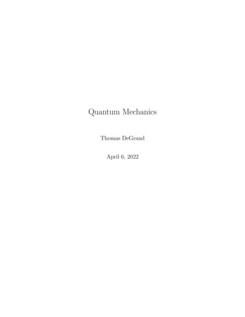
A Textbook of Physical Chemistry – Volume I34Besides the record of different operators presented in ‘Table 2’, there still many operators which areextremely important like angular momentum, parity, or the step-up–step-down operators. The discussion ofevery operator is beyond the scope of this book; however, a brief discussion of the essential operators inquantum mechanics is given below.1. Angular momentum operator: In order to understand the angular momentum operator in the quantummechanical world, we first need to understand the classical mechanics of one particle angular momentum. Letus consider a particle of mass m which moves within a cartesian coordinate system with a position vector “r”.Hence, we can say that𝑟 𝑖𝑥 𝑗𝑦 𝑘𝑧(97)The coordinates x. y and z are the functions of time, and therefore, we can define the velocity as the timederivative of the position vector as given below.𝑣 𝑑𝑟𝑑𝑥𝑑𝑦𝑑𝑧 𝑖 𝑗 𝑘𝑑𝑡𝑑𝑡𝑑𝑡𝑑𝑡(98)or𝑣 𝑣𝑥 𝑣𝑦 𝑣𝑧(99)Now, since we that p mv, we can say that𝑝𝑥 𝑚𝑣𝑥 ; 𝑝𝑦 𝑚𝑣𝑦 ;𝑝𝑧 𝑚𝑣𝑧(100)The angular momentum of a particle with mass m and distance r from the origin is given by the followingrelation.Figure 6. The angular momentum vector.𝐿⃗ 𝑣 𝑚 𝑟Buy the complete book with TOC navigation,high resolution images andno watermark.Copyright Mandeep Dalal(101)
CHAPTER 1 Quantum Mechanics – I35(102)𝐿⃗ 𝑝 𝑟Equation (102) can also be written in the form of a matrix as:𝑖𝑥𝐿 [𝑝𝑥𝐿𝑥 𝑦𝑝𝑧 𝑧𝑝𝑦 ;𝑗𝑦𝑝𝑦𝑘𝑧]𝑝𝑧𝐿𝑦 𝑧𝑝𝑥 𝑥𝑝𝑧 ; 𝐿𝑧 𝑥𝑝𝑦 𝑦𝑝𝑥(103)(104)Where i, j, k are the unit vectors along x, y, z axis and Lx, Ly, Lz are the component of angular momentum alongx, y, z axis. Moreover, it is also worthy to note that the angular momentum vector is always perpendicular tothe direction of the position vector of the particle i.e. the plane in which the particle is moving.Now since the mathematical nature of any quantum mechanical operator is dependent upon theclassical expression of the same observable, the angular momentum is not any exception. The quantummechanical operator for angular momentum is given below.𝐿̂ 𝑖ℎ(𝑟 ) 𝑖ħ(𝑟 )2𝜋(105)The angular momentum can be divided into two categories; one is orbital angular momentum (due to the orbitalmotion of the particle) and the other is spin angular momentum (due to spin motion of the particle). Moreover,being a vector quantity, the operator of angular momentum can also be resolved along different axes.𝐿̂ 𝐿̂𝑥 𝐿̂𝑦 𝐿̂𝑧(106)ℎ ℎ ℎ 𝐿̂𝑥 𝑦𝑝𝑧 𝑧𝑝𝑦 𝑦 () 𝑧() (𝑦 𝑧 )2𝜋𝑖 𝑧2𝜋𝑖 𝑦2𝜋𝑖 𝑧 𝑦(107)ℎ ℎ ℎ 𝐿̂𝑦 𝑧𝑝𝑥 𝑥𝑝𝑧 𝑧 () 𝑥() (𝑧 𝑥 )2𝜋𝑖 𝑥2𝜋𝑖 𝑧2𝜋𝑖 𝑥 𝑧(108)ℎ ℎ ℎ 𝐿̂𝑧 𝑥𝑝𝑦 𝑦𝑝𝑥 𝑥 () 𝑦() (𝑥 𝑦 )2𝜋𝑖 𝑦2𝜋𝑖 𝑥2𝜋𝑖 𝑦 𝑥(109)And we know thatoror𝐿̂ ℎ 𝑥 ) (𝑥 𝑦 )][(𝑦 𝑧 ) (𝑧2𝜋𝑖 𝑧 𝑦 𝑥 𝑧 𝑦 𝑥(110)It is also worthy to recall that equation (107) to (110) can also be reported in terms of ħ; or by multiplying anddividing by i, or both.Buy the complete book with TOC navigation,high resolution images andno watermark.Copyright Mandeep Dalal
A Textbook of Physical Chemistry – Volume I362. Ladder operator: These operators are also called as step-up–step-down or rising-lowering operators. Thereason for such terminology lies in the fact that these operators can increase or decrease the eigenvalues.Moreover, it should also be noted that this increase or decrease is always quantized in nature.𝐽̂ 𝐽̂𝑥 𝑖𝐽̂𝑦(111)𝐽̂ 𝐽̂𝑥 𝑖𝐽̂𝑦(112)andThe equation (111) and (112) represent the step-up and step-down operators respectively. These operators canbe used to increase or decrease the eigen values. Operator EvaluationThe operator evaluation simply means that we need to find the result by applying the operator over agiven function. Some general examples are given below.i) (d/dx) (x5): In this case d/dx is the operator while the function x5 is the operand.𝑑 5𝑥 5𝑥 4𝑑𝑥(113)ii) ʃ(x5): In this case, ʃ is the operator while the function x5 is the operand. 𝑥5 𝑥66(114)iii) (d2/dt2) (ASine 2πνt): In this particular case, (d2/dt2) is the operator while the function (A Sin 2πνt) is theoperand.Let the function is symbolized by y. Then, we have𝑦 𝐴 𝑆𝑖𝑛 2𝜋𝜈𝑡(115)𝑑𝑦 𝐴 2𝜋𝜈 𝐶𝑜𝑠 2𝜋𝜈𝑡𝑑𝑡(116)𝑑2 𝑦 𝐴 4𝜋 2 𝜈 2 𝑆𝑖𝑛 2𝜋𝜈𝑡𝑑𝑡 2(117)Differentiating with respect to t, we getDifferentiating againThe operator evaluation is frequently used as a part of the commutator calculation and will bediscussed in detail in this chapter.Buy the complete book with TOC navigation,high resolution images andno watermark.Copyright Mandeep Dalal
CHAPTER 1 Quantum Mechanics – I37 Calculation of Resultant OperatorSometimes the operator is simplified to another form which is easy to apply over a function. Thisresultant operator is obtained by the rules of operator algebra. For instance, consider the following cases.i) Find the resultant expression for the following operator2𝑑( 𝑥)𝑑𝑥(118)In order to find the resultant operator, suppose a function ψ(x) which is used as an operand, then we can say2𝑑𝑑𝑑𝑥) 𝜓 ( 𝑥) ( 𝑥) 𝜓𝑑𝑥𝑑𝑥𝑑𝑥(119)2𝑑𝑑𝑑( 𝑥) 𝜓 ( 𝑥) ( ���𝑑𝜓𝑑𝑥𝑥) 𝜓 ( 𝑥) (𝑥 𝜓 �𝜓𝑥) 𝜓 (𝑥 2 𝑥𝜓)𝑑𝑥𝑑𝑥𝑑𝑥(122)(2𝑑𝑑2 𝜓 𝑑𝜓𝑑𝜓𝑑𝑥( 𝑥) 𝜓 [𝑥 2 2 (2𝑥)] [𝑥 𝜓 �𝑑2 𝜓𝑑𝜓𝑑𝜓2( 𝑥) 𝜓 𝑥 2𝑥 𝑥 𝜓𝑑𝑥𝑑𝑥 2𝑑𝑥𝑑𝑥(124)(2𝑑𝑑2𝑑𝑥) 𝜓 [𝑥 2 2 3𝑥 1] 𝜓𝑑𝑥𝑑𝑥𝑑𝑥(125)Removing ψ from both sides, we get2𝑑𝑑2𝑑( 𝑥) 𝑥 2 2 3𝑥 1𝑑𝑥𝑑𝑥𝑑𝑥(126)ii) Find the resultant expression for the following operator(𝑥 𝑑 𝑑)𝑑𝑥 𝑑𝑥(127)In order to find the resultant operator, suppose a function ψ(x) which is used as operand, then we can say thatBuy the complete book with TOC navigation,high resolution images andno watermark.Copyright Mandeep Dalal
A Textbook of Physical Chemistry – Volume I38[(𝑥 𝑑 𝑑𝑑 𝑑𝜓) ] 𝜓 (𝑥 )𝑑𝑥 𝑑𝑥𝑑𝑥 𝑑𝑥[(𝑥 𝑑 𝑑𝑑𝜓 𝑑2 𝜓) ]𝜓 𝑥 𝑑𝑥 𝑑𝑥𝑑𝑥 𝑑𝑥 2(128)Removing ψ from both sides, we get(𝑥 𝑑 𝑑𝑑𝑑2) 𝑥 2𝑑𝑥 𝑑𝑥𝑑𝑥 𝑑𝑥(129)iii) Find the resultant expression for the following operator2𝑑( 𝑥)𝑑𝑥(130)In order to find the resultant operator, suppose a function ψ(x) which is used as operand, then we can say that2𝑑𝑑𝑑[( 𝑥) ] 𝜓 [( 𝑥) ( 𝑥)] 𝜓𝑑𝑥𝑑𝑥𝑑𝑥[(2𝑑𝑑𝑑𝜓 𝑥) ] 𝜓 ( 𝑥) ( 𝑥𝜓)𝑑𝑥𝑑𝑥𝑑𝑥2𝑑𝑑2 𝜓 𝑑𝑑𝜓[( 𝑥) ] 𝜓 𝑥𝜓 𝑥 ���2 𝜓𝑑𝜓𝑑𝑥𝑑𝜓 𝑥) ] 𝜓 𝑥 𝜓 𝑥 2𝑑𝑑2 𝜓𝑑𝜓[( 𝑥) ] 𝜓 2𝑥 𝑥2𝜓 135)Removing ψ from both sides, we get2𝑑𝑑2𝑑( 𝑥) 2 2𝑥 𝑥2 1𝑑𝑥𝑑𝑥𝑑𝑥(136)iv) Find the resultant expression for the following operator(𝑥 𝑑𝑑) (𝑥 )𝑑𝑥𝑑𝑥(137)In order to find the resultant operator, suppose a function ψ(x) which is used as operand, then we can say thatBuy the complete book with TOC navigation,high resolution images andno watermark.Copyright Mandeep Dalal
CHAPTER 1 Quantum Mechanics – I𝑑𝑑𝑑𝑑𝜓) (𝑥 )] 𝜓 (𝑥 ) (𝑥𝜓 𝜓 𝑑𝑑2 𝜓) (𝑥 )] 𝜓 𝑥𝑥𝜓 𝑥 𝑥𝜓 2𝑑𝑥𝑑𝑥𝑑𝑥 ��� 𝑑2 𝜓) (𝑥 )] 𝜓 𝑥 2 𝜓 𝑥 𝑥 𝜓 𝑑𝑥𝑑𝑥𝑑𝑥𝑑𝑥𝑑𝑥 𝑑𝑥 2(140)[(𝑥 𝑑𝑑𝑑𝑥 𝑑2 𝜓) (𝑥 )] 𝜓 𝑥 2 𝜓 𝜓 𝑑𝑥𝑑𝑥𝑑𝑥 𝑑𝑥 2(141)[(𝑥 𝑑𝑑𝑑𝑥𝑑2) (𝑥 )] 𝜓 [𝑥 2 2] 𝜓𝑑𝑥𝑑𝑥𝑑𝑥 𝑑𝑥(142)𝑑𝑑𝑑2) (𝑥 ) 𝑥 2 1 2𝑑𝑥𝑑𝑥𝑑𝑥(143)[(𝑥 [(𝑥 [(𝑥 39Removing ψ from both sides, we get(𝑥 The resultant operator calculation is frequently used as a part of the commutator calculation and willbe discussed in detail in this chapter. Commutation Relations of Various Quantum Mechanical OperatorsAs we have discussed previously that one of the most fundamental properties of operatormultiplication is the commutation relation or the commutation rule. two operators, A and B, are said to becommutating or non-commutating depending upon the value of their commutator.̂ 𝐵̂] 𝐴̂𝐵̂ 𝐵̂𝐴̂ 0 (144)̂ 𝐵̂] 𝐴̂𝐵̂ 𝐵̂𝐴̂ 0 ���𝑔[𝐴,(145)The physical significance of the commutation relations is that when two operators commute, it means they arehaving a simultaneous set of eigenfunctions; and their corresponding physical properties can be calculatedsimultaneously and accurately. However, if the commutator is non-zero, the respective physical propertiescannot be obtained simultaneously and accurately. Some important commutation relations are given below.1. Commutators of some simple operators:i) Calculate the commutator of the following[𝑥,𝑑]𝑑𝑥Let it be operated over a function ψ. We haveBuy the complete book with TOC navigation,high resolution images andno watermark.Copyright Mandeep Dalal(146)
A Textbook of Physical Chemistry – Volume I40𝑑𝑑𝑑𝜓 𝑥𝜓]𝜓 ��� 𝜓 𝑥]𝜓 𝑥𝑑𝑥𝑑𝑥𝑑𝑥(148)𝑑] 𝜓 𝜓𝑑𝑥(149)𝑑] 1𝑑𝑥(150)𝑑]𝑑𝑥(151)𝑑𝑑𝑑𝜓 𝑦𝜓]𝜓 ���𝑑𝑦 𝑦 𝜓]𝜓 𝑦𝑑𝑥𝑑𝑥𝑑𝑥𝑑𝑥(153)𝑑]𝜓 0𝑑𝑥(154)[𝑥,[𝑥,[𝑥,or[𝑥,ii) Calculate the commutator of the following[𝑦,Let it be operated over a function ψ. We have[𝑦,[𝑦,[𝑥,iii) Calculate the commutator of the following𝑑 𝑑2[ , 2]𝑑𝑥 𝑑𝑥(155)𝑑 𝑑2𝑑 𝑑2𝑑2 𝑑[ , 2 ]𝜓 𝜓 𝜓𝑑𝑥 𝑑𝑥𝑑𝑥 𝑑𝑥 2𝑑𝑥 2 𝑑𝑥(156)𝑑 𝑑2𝑑3 𝜓 𝑑3 𝜓[ , 2 ]𝜓 𝑑𝑥 𝑑𝑥𝑑𝑥 3 𝑑𝑥 3(157)𝑑 𝑑2[ , 2 ]𝜓 0𝑑𝑥 𝑑𝑥(158)Let it be operated over a function ψ. We haveorBuy the complete book with TOC navigation,high resolution images andno watermark.Copyright Mandeep Dalal
CHAPTER 1 Quantum Mechanics – I412. Commutators of position and linear momentum operators:i) Find the commutator of the following[𝑥̂, 𝑝̂𝑥 ](159)[𝑥̂, 𝑝̂𝑥 ]𝜓 𝑥̂ 𝑝̂𝑥 𝜓 𝑝̂𝑥 ̂𝑥 𝜓(160)Let it be operated over a function ψ. We have[𝑥̂, 𝑝̂𝑥 ]𝜓 𝑥[𝑥̂, 𝑝̂𝑥 ]𝜓 ℎ ℎ 𝜓 𝑥𝜓2𝜋𝑖 𝑥2𝜋𝑖 𝑥ℎ 𝜓ℎ 𝜓ℎ 𝑥𝑥 𝑥 𝜓2𝜋𝑖 𝑥 2𝜋𝑖 𝑥2𝜋𝑖 𝑥[𝑥̂, 𝑝̂𝑥 ]𝜓 [𝑥̂, 𝑝̂𝑥 ] (161)(162)ℎ𝜓2𝜋𝑖ℎℎ𝑖 𝑖ħ2𝜋𝑖 2𝜋(163)ii) Find the commutator of the following[𝑥̂ 𝑛 , 𝑝̂𝑥 ](164)[𝑥̂ 𝑛 , 𝑝̂𝑥 ]𝜓 𝑥̂ 𝑛 𝑝̂𝑥 𝜓 𝑝̂𝑥 𝑥̂ 𝑛 𝜓(165)Let it be operated over a function ψ. We have[𝑥̂ 𝑛 , 𝑝̂𝑥 ]𝜓 𝑥 𝑛[𝑥̂ 𝑛 , 𝑝̂𝑥 ]𝜓 ℎ ℎ 𝑛𝜓 𝑥 𝜓2𝜋𝑖 𝑥2𝜋𝑖 𝑥ℎ 𝑛 𝜓ℎ 𝑛 𝜓ℎ𝑥 𝑥 𝑛𝑥 𝑛 1 𝜓2𝜋𝑖 𝑥 2𝜋𝑖 𝑥2𝜋𝑖[𝑥̂ 𝑛 , 𝑝̂𝑥 ]𝜓 (166)(167)ℎ𝑛𝑥 𝑛 1 𝜓2𝜋𝑖(168)ℎ𝑛𝑥 𝑛 12𝜋𝑖(169)Removing ψ from both sides, we get[𝑥̂ 𝑛 , 𝑝̂𝑥 ] The commutation relations between position and linear momentum can mainly be divided into threecategories as discussed below.(a) When position and momentum are along the same axis:[𝑥̂ 𝑛 , 𝑝̂𝑥 ] 𝑛𝑖ħ𝑥 𝑛 1Buy the complete book with TOC navigation,high resolution images andno watermark.Copyright Mandeep Dalal(170)
A Textbook of Physical Chemistry – Volume I42[ 𝑝̂𝑥 , 𝑥̂ 𝑛 ] 𝑛𝑖ħ𝑥 𝑛 1(171)[𝑥̂, 𝑝̂𝑥𝑛 ] 𝑛𝑖ħ𝑝𝑥𝑛 1(172)[𝑝̂𝑥𝑛 , 𝑥̂ ] 𝑛𝑖ħ𝑝𝑥𝑛 1(173)and(b) When position and momentum are along different axis:[𝑥̂, 𝑝̂𝑦 ] 0(174)[𝑥̂, 𝑝̂𝑧 ] 0(175)[𝑦̂, 𝑝̂𝑥 ] 0(176)[𝑦̂, 𝑝̂𝑧 ] 0(177)[𝑧̂ , 𝑝̂𝑥 ] 0(178)[𝑧̂ , 𝑝̂𝑦 ] 0(179)[𝑥̂, 𝑦̂] 0(180)[𝑥̂, 𝑧̂ ] 0(181)[𝑦̂, 𝑧̂ ] 0(182)[𝑝̂𝑥 , 𝑝̂𝑦 ] 0(183)[𝑝̂𝑥 , 𝑝̂𝑧 ] 0(184)[𝑝̂𝑦 , 𝑝̂𝑧 ] 0(185)(b) When positions are along the different axis:(b) When positions are along the different axis:3. Commutators of angular momentum operators:i) The commutator of orbital angular momentum operators along x and y-axis.[𝐿̂𝑥 , 𝐿̂𝑦 ] 𝐿̂𝑥 𝐿̂𝑦 𝐿̂𝑦 𝐿̂𝑥(186)Finding the values of 𝐿̂𝑥 𝐿̂𝑦 , we get𝐿̂𝑥 𝐿̂𝑦 [Buy the complete book with TOC navigation,high resolution images andno watermark.ℎ ℎ (𝑦 𝑧 )] [(𝑧 𝑥 )]2𝜋𝑖 𝑧 𝑦 2𝜋𝑖 𝑥 𝑧Copyright Mandeep Dalal(187)
CHAPTER 1 Quantum Mechanics – I43ℎ2 2 [(𝑦 𝑧 ) (𝑧 𝑥 )]4𝜋 𝑧 𝑦 𝑥 𝑧(188)ℎ2 2 (𝑦 𝑧 𝑧 𝑧 𝑦 𝑥 𝑧 𝑥 )4𝜋 𝑧 𝑥 𝑦 𝑥 𝑧 𝑧 𝑦 𝑧(189)ℎ2 𝑧 2 2 2 22 2 (𝑦 𝑦𝑧 2 𝑧 2 𝑦𝑥 2 𝑧𝑥)4𝜋 𝑥 𝑧 𝑧𝑥 𝑦𝑥 𝑧 𝑦𝑧(190) ħ2 (𝑦 2 2 2 2 𝑦𝑧 2 𝑧 2 2 𝑦𝑥 2 𝑧𝑥) 𝑥 𝑧𝑥 𝑦𝑥 𝑧 𝑦𝑧(191)Similarly obtaining the value of 𝐿̂𝑦 𝐿̂𝑥 , we getℎ ℎ (𝑧 𝑥 )] [(𝑦 𝑧 )]2𝜋𝑖 𝑥 𝑧 2𝜋𝑖 𝑧 𝑦(192)ℎ2 𝑥 ) (𝑦 𝑧 )][(𝑧24𝜋 𝑥 𝑧 𝑧 𝑦(193)ℎ2 (𝑧 𝑦 𝑧 𝑧 𝑥 𝑦 𝑥 𝑧 )24𝜋 𝑥 𝑧 𝑥 𝑦 𝑧 𝑧 𝑧 𝑦(194)ℎ2 2 2 2 2 𝑧2 𝑧 𝑥𝑦 𝑥𝑧 𝑥(𝑧𝑦)22224𝜋 𝑥𝑧 𝑥𝑦 𝑧 𝑧𝑦 𝑦 𝑧(195)𝐿̂𝑦 𝐿̂𝑥 [ 2 2 2 2 2 ħ (𝑧𝑦 2 𝑧 2 𝑥𝑦 2 𝑥𝑧 𝑥 ) 𝑥𝑧 𝑥𝑦 𝑧 𝑧𝑦 𝑦2(196)Now putting the values of 𝐿̂𝑥 𝐿̂𝑦 and 𝐿̂𝑦 𝐿̂𝑥 in equation (183), we get the following.[𝐿̂𝑥 , 𝐿̂𝑦 ] [ ħ2 (𝑦 2 2 2 2 𝑦𝑧 2 𝑧 2 2 𝑦𝑥 2 𝑧𝑥)] 𝑥 𝑧𝑥 𝑦𝑥 𝑧 𝑦𝑧 [ ħ2 (𝑧𝑦(197) 2 2 2 2 2 𝑧 𝑥𝑦 𝑥𝑧 𝑥 )]222 𝑥𝑧 𝑥𝑦 𝑧 𝑧𝑦 𝑦[𝐿̂𝑥 , 𝐿̂𝑦 ] ħ2 (𝑦 𝑥 ) 𝑥 𝑦(198)Taking negative sign common, we get[𝐿̂𝑥 , 𝐿̂𝑦 ] ħ2 (𝑥Buy the complete book with TOC navigation,high resolution images andno watermark. 𝑦 ) 𝑦 𝑥Copyright Mandeep Dalal(199)
A Textbook of Physical Chemistry – Volume I44[𝐿̂𝑥 , 𝐿̂𝑦 ] 𝑖ħ [ 𝑖ħ (𝑥 𝑦 )] 𝑦 𝑥[𝐿̂𝑥 , 𝐿̂𝑦 ] 𝑖ħ𝐿̂𝑧(200)(201)ii) The commutator of orbital angular momentum operators along y and z-axis.[𝐿̂𝑦 , 𝐿̂𝑧 ] 𝐿̂𝑦 𝐿̂𝑧 𝐿̂𝑧 𝐿̂𝑦(202)Finding the values of 𝐿̂𝑦 𝐿̂𝑧 , we get𝐿̂𝑦 𝐿̂𝑧 [ℎ ℎ (𝑧 𝑥 )] [(𝑥 𝑦 )]2𝜋𝑖 𝑥 𝑧 2𝜋𝑖 𝑦 𝑥(203)ℎ2 2 [(𝑧 𝑥 ) (𝑥 𝑦 )]4𝜋 𝑥 𝑧 𝑦 𝑥(204)ℎ2 2 (𝑧 𝑥 𝑥 𝑥 𝑧 𝑦 𝑥 𝑦 )4𝜋 𝑥 𝑦 𝑧 𝑦 𝑥 𝑥 𝑧 𝑥(205)ℎ2 𝑥 2 2 22 2 (𝑧 𝑧𝑥 𝑥 2 𝑧𝑦 2 𝑥𝑦)4𝜋 𝑦 𝑥 𝑥𝑦 𝑧𝑦 𝑥 𝑧𝑥(206) ħ2 (𝑧 2 2 2 𝑧𝑥 𝑥 2 2 𝑧𝑦 2 𝑥𝑦) 𝑦 𝑥𝑦 𝑧𝑦 𝑥 𝑧𝑥(207)Similarly obtaining the value of 𝐿̂𝑧 𝐿̂𝑦 , we getℎ ℎ (𝑥 𝑦 )] [(𝑧 𝑥 )]2𝜋𝑖 𝑦 𝑥 2𝜋𝑖 𝑥 𝑧(208)ℎ2 𝑦 ) (𝑧 𝑥 )][(𝑥24𝜋 𝑦 𝑥 𝑥 𝑧(209)ℎ2 (𝑥 𝑧 𝑥 𝑥 𝑦 𝑧 𝑦 𝑥 )24𝜋 𝑦 𝑥 𝑦 𝑧 𝑥 𝑥 𝑥 𝑧(210)ℎ2 2 2 2 2 𝑥2 𝑥 𝑦𝑧 𝑦𝑥 𝑦(𝑥𝑧)224𝜋 𝑦𝑥 𝑦𝑧 𝑥 𝑥𝑧 𝑧 𝑥(211)𝐿̂𝑧 𝐿̂𝑦 [ 2 2 2 2 2 ħ (𝑥𝑧 𝑥 𝑦𝑧 2 𝑦𝑥 𝑦 ) 𝑦𝑥 𝑦𝑧 𝑥 𝑥𝑧 𝑧2Now putting the values of 𝐿̂𝑦 𝐿̂𝑧 and 𝐿̂𝑧 𝐿̂𝑦 in equation (212), we get the following.Buy the complete book with TOC navigation,high resolution images andno watermark.Copyright Mandeep Dalal(212)
CHAPTER 1 Quantum Mechanics – I[𝐿̂𝑦 , 𝐿̂𝑧 ] [ ħ2 (𝑧45 2 2 22 𝑧𝑥 𝑥 2 𝑧𝑦 2 𝑥𝑦)] 𝑦 𝑥𝑦 𝑧𝑦 𝑥 𝑧𝑥 [ ħ2 (𝑥𝑧(213) 2 2 2 2 𝑥2 𝑦𝑧 2 𝑦𝑥 𝑦 )] 𝑦𝑥 𝑦𝑧 𝑥 𝑥𝑧 𝑧 𝑦 ) 𝑦 𝑧(214) 𝑧 ) 𝑧 𝑦(215)[𝐿̂𝑦 , 𝐿̂𝑧 ] ħ2 (𝑧Taking negative sign common, we get[𝐿̂𝑦 , 𝐿̂𝑧 ] ħ2 (𝑦[𝐿̂𝑦 , 𝐿̂𝑧 ] 𝑖ħ [ 𝑖ħ (𝑦 𝑧 )] 𝑧 𝑦[𝐿̂𝑦 , 𝐿̂𝑧 ] 𝑖ħ𝐿̂𝑥(216)(217)iii) The commutator of orbital angular momentum operators along z and x-axis.[𝐿̂𝑧 , 𝐿̂𝑥 ] 𝐿̂𝑧 𝐿̂𝑥 𝐿̂𝑥 𝐿̂𝑧(218)Finding the values of 𝐿̂𝑧 𝐿̂𝑥 , we getℎ ℎ (𝑥 𝑦 )] [(𝑦 𝑧 )]2𝜋𝑖 𝑦 𝑥 2𝜋𝑖 𝑧 𝑦(219)ℎ2 𝑦 ) (𝑦 𝑧 )][(𝑥24𝜋 𝑦 𝑥 𝑧 𝑦(220)ℎ2 (𝑥 𝑦 𝑥 𝑧 𝑦 𝑦 𝑦 𝑧 )24𝜋 𝑦 𝑧 𝑦 𝑦 𝑥 𝑧 𝑥 𝑦(221)ℎ2 𝑦 2 2 2 22 𝑥𝑦 𝑥𝑧 𝑦 𝑦𝑧(𝑥)4𝜋 2 𝑧 𝑦 𝑦𝑧 𝑦 2 𝑥𝑧 𝑥𝑦(222)𝐿̂𝑧 𝐿̂𝑥 [ ħ2 (𝑥 2 2 2 2 𝑥𝑦 𝑥𝑧 2 𝑦 2 𝑦𝑧) 𝑧 𝑦𝑧 𝑦 𝑥𝑧 𝑥𝑦(223)Similarly obtaining the value of 𝐿̂𝑥 𝐿̂𝑧 , we get𝐿̂𝑥 𝐿̂𝑧 [Buy the complete book with TOC navigation,high resolution images andno watermark.ℎ ℎ (𝑦 𝑧 )] [(𝑥 𝑦 )]2𝜋𝑖 𝑧 𝑦 2𝜋𝑖 𝑦 𝑥Copyright Mandeep Dalal(224)
A Textbook of Physical Chemistry – Volume I46ℎ2 2 [(𝑦 𝑧 ) (𝑥 𝑦 )]4𝜋 𝑧 𝑦 𝑦 𝑥(225)ℎ2 2 (𝑦 𝑥 𝑦 𝑦 𝑧 𝑥 𝑧 𝑦 )4𝜋 𝑧 𝑦 𝑧 𝑥 𝑦 𝑦 𝑦 𝑥(226)ℎ2 2 2 2 𝑦 22 2 (𝑦𝑥 𝑦 𝑧𝑥 2 𝑧 𝑧𝑦)4𝜋 𝑧𝑦 𝑧𝑥 𝑦 𝑥 𝑦 𝑦𝑥(227)or ħ2 (𝑦𝑥 2 2 2 2 𝑦2 𝑧𝑥 2 𝑧 𝑧𝑦) 𝑧𝑦 𝑧𝑥 𝑦 𝑥 𝑦𝑥(228)Now putting the values of 𝐿̂𝑧 𝐿̂𝑥 and 𝐿̂𝑥 𝐿̂𝑧 in equation (218), we get the following.[𝐿̂𝑧 , 𝐿̂𝑥 ] [ ħ2 (𝑥 2 2 2 2 𝑥𝑦 𝑥𝑧 2 𝑦 2 𝑦𝑧)] 𝑧 𝑦𝑧 𝑦 𝑥𝑧 𝑥𝑦(229) 2 2 2 22 [ ħ (𝑦𝑥 𝑦 𝑧𝑥 2 𝑧 𝑧𝑦)] 𝑧𝑦 𝑧𝑥 𝑦 𝑥 𝑦𝑥2[𝐿̂𝑧 , 𝐿̂𝑥 ] ħ2 (𝑥 𝑧 ) 𝑧 𝑥(230)Taking negative sign common, we get[𝐿̂𝑧 , 𝐿̂𝑥 ] ħ2 (𝑦 𝑧 ) 𝑧 𝑦[𝐿̂𝑧 , 𝐿̂𝑥 ] 𝑖ħ [ 𝑖ħ (𝑦 𝑧 )] 𝑧 𝑦[𝐿̂𝑧 , 𝐿̂𝑥 ] 𝑖ħ𝐿̂𝑦(231)(232)(233)iv) The commutator of total orbital angular momentum squared operator and orbital angular momentum alongone of the three-axis.[𝐿̂2 , 𝐿̂𝑧 ] [𝐿̂2𝑥 𝐿̂2𝑦 𝐿̂2𝑧 , 𝐿̂𝑧 ](234) [𝐿̂2𝑥 𝐿̂𝑧 𝐿̂2𝑦 𝐿̂𝑧 𝐿̂2𝑧 𝐿̂𝑧 𝐿̂𝑧 𝐿̂2𝑥 𝐿̂𝑧 𝐿̂2𝑦 𝐿̂𝑧 𝐿̂2𝑧 ](235) [(𝐿̂2𝑥 𝐿̂𝑧 𝐿̂𝑧 𝐿̂2𝑥 ) (𝐿̂2𝑦 𝐿̂𝑧 𝐿̂𝑧 𝐿̂2𝑦 ) (𝐿̂2𝑧 𝐿̂𝑧 𝐿̂𝑧 𝐿̂2𝑧 )](236)[𝐿̂2 , 𝐿̂𝑧 ] [𝐿̂2𝑥 , 𝐿̂𝑧 ] [𝐿̂2𝑦 𝐿̂𝑧 ] [𝐿̂2𝑧 𝐿̂𝑧 ](237)Now finding [𝐿̂2𝑥 , 𝐿̂𝑧 ] first, we getBuy the complete book with TOC navigation,high resolution images andno watermark.Copyright Mandeep Dalal
CHAPTER 1 Quantum Mechanics – I47[𝐿̂2𝑥 , 𝐿̂𝑧 ] 𝐿̂2𝑥 𝐿̂𝑧 𝐿̂𝑧 𝐿̂2𝑥(238) 𝐿̂𝑥 𝐿̂𝑥 𝐿̂𝑧 𝐿̂𝑧 𝐿̂𝑥 𝐿̂𝑥(239) [𝐿̂𝑥 𝐿̂𝑥 𝐿̂𝑧 𝐿̂𝑥 𝐿̂𝑧 𝐿̂𝑥 ] [𝐿̂𝑧 𝐿̂𝑥 𝐿̂𝑥 𝐿̂𝑥 𝐿̂𝑧 𝐿̂𝑥 ](240) 𝐿̂𝑥 [𝐿̂𝑥 𝐿̂𝑧 𝐿̂𝑧 𝐿̂𝑥 ] [𝐿̂𝑧 𝐿̂𝑥 𝐿̂𝑥 𝐿̂𝑧 ]𝐿̂𝑥(241) 𝐿̂𝑥 [𝐿̂𝑥 𝐿̂𝑧 𝐿̂𝑧 𝐿̂𝑥 ] [𝐿̂𝑥 𝐿̂𝑧 𝐿̂𝑧 𝐿̂𝑥 ]𝐿̂𝑥(242) 𝐿̂𝑥 [ 𝑖ħ𝐿̂𝑦 ] [ 𝑖ħ𝐿̂𝑦 ]𝐿̂𝑥(243) 𝑖ħ𝐿̂𝑥 𝐿̂𝑦 𝑖ħ𝐿̂𝑦 𝐿̂𝑥 𝑖ħ[𝐿̂𝑥 𝐿̂𝑦 𝐿̂𝑦 𝐿̂𝑥 ](244)[𝐿̂2𝑦 , 𝐿̂𝑧 ] 𝐿̂2𝑦 𝐿̂𝑧 𝐿̂𝑧 𝐿̂2𝑦(245) 𝐿̂𝑦 𝐿̂𝑦 𝐿̂𝑧 𝐿̂𝑧 𝐿̂𝑦 𝐿̂𝑦(246)Similarly, [𝐿̂𝑦 𝐿̂𝑦 𝐿̂𝑧 𝐿̂𝑦 𝐿̂𝑧 𝐿̂𝑦 ] [𝐿̂𝑧 𝐿̂𝑦 𝐿̂𝑦 𝐿̂𝑦 𝐿̂𝑧 𝐿̂𝑦 ] 𝐿̂𝑦 [𝐿̂𝑦 𝐿̂𝑧 𝐿̂𝑧 𝐿̂𝑦 ] [𝐿̂𝑧 𝐿̂𝑦 𝐿̂𝑦 𝐿̂𝑧 ]𝐿̂𝑦 𝐿̂𝑦 [𝐿̂𝑦 𝐿̂𝑧 𝐿̂𝑧 𝐿̂𝑦 ] [𝐿̂𝑦 𝐿̂𝑧 𝐿̂𝑧 𝐿̂𝑦 ]𝐿̂𝑦 𝐿̂𝑦 [𝑖ħ𝐿̂𝑥 ] [𝑖ħ𝐿̂𝑥 ]𝐿̂𝑦 𝑖ħ𝐿̂𝑦 𝐿̂𝑥 𝑖ħ𝐿̂𝑥 𝐿̂𝑦 𝑖ħ[𝐿̂𝑦 𝐿̂𝑥 𝐿̂𝑥 𝐿̂𝑦 ](247)Similarly,[𝐿̂2𝑧 , 𝐿̂𝑧 ] 𝐿̂2𝑧 𝐿̂𝑧 𝐿̂𝑧 𝐿̂2𝑧 𝐿̂𝑧 𝐿̂𝑧 𝐿̂𝑧 𝐿̂𝑧 𝐿̂𝑧 𝐿̂𝑧[𝐿̂2𝑧 , 𝐿̂𝑧 ] 0(248)Now putting the value of 𝐿̂2𝑥 𝐿̂𝑧 , 𝐿̂2𝑦 𝐿̂𝑧 and 𝐿̂2𝑧 𝐿̂𝑧 in equation (237), we get[𝐿̂2 , 𝐿̂𝑧 ] 𝑖ħ[𝐿̂𝑥 𝐿̂𝑦 𝐿̂𝑦 𝐿̂𝑥 ] 𝑖ħ[𝐿̂𝑦 𝐿̂𝑥 𝐿̂𝑥 𝐿̂𝑦 ] 0[𝐿̂2 , 𝐿̂𝑧 ] 0AlsoBuy the complete book with TOC navigation,high resolution images andno watermark.Copyright Mandeep Dalal(249)
A Textbook of Physical Chemistry – Volume I48[𝐿̂2 , 𝐿̂𝑦 ] 0; 𝑎𝑛𝑑 [𝐿̂2 , 𝐿̂𝑥 ] 0(250)Hence, the commutation relations of angular momentum operators along two different directions do notcommute with each other and hence cannot give eigenvalues simultaneously and accurately. One the otherhand, total angular momentum squared and angular momentum along one axis do commute with each other.The commutation relations between angular momentum operators can be mainly divided into fourcategories as discussed below.(a) Orbital angular momentum commutation:[𝐿̂𝑥 , 𝐿̂𝑦 ] 𝑖ħ𝐿̂𝑧 ;[𝐿̂𝑦 , 𝐿̂𝑥 ] 𝑖ħ𝐿̂𝑧(251)[𝐿̂𝑦 , 𝐿̂𝑧 ] 𝑖ħ𝐿̂𝑥 ;[𝐿̂𝑧 , 𝐿̂𝑦 ] 𝑖ħ𝐿̂𝑥(252)[𝐿̂𝑧 , 𝐿̂𝑥 ] 𝑖ħ𝐿̂𝑦 ;[𝐿̂𝑥 , 𝐿̂𝑧 ] 𝑖ħ𝐿̂𝑦(253)[𝐿̂2 , 𝐿̂𝑥 ] 0;[𝐿̂𝑥 , 𝐿̂2 ] 0(254)[𝐿̂2 , 𝐿̂𝑦 ] 0;[𝐿̂𝑦 , 𝐿̂2 ] 0(255)[𝐿̂2 , 𝐿̂𝑧 ] 0;[𝐿̂𝑧 , 𝐿̂2 ] 0(256)(b) Spin angular momentum commutation:[𝑆̂𝑥 , 𝑆̂𝑦 ] 𝑖ħ𝑆̂𝑧 ;[𝑆̂𝑦 , 𝑆̂𝑥 ] 𝑖ħ𝑆̂𝑧(257)[𝑆̂𝑦 , 𝑆̂𝑧 ] 𝑖ħ𝑆̂𝑥 ;[𝑆̂𝑧 , 𝑆̂𝑦 ] 𝑖ħ𝑆̂𝑥(258)[𝑆̂𝑧 , 𝑆̂𝑥 ] 𝑖ħ𝑆̂𝑦 ;[𝑆̂𝑥 , 𝑆̂𝑧 ] 𝑖ħ𝑆̂𝑦(259)[𝑆̂ 2 , 𝑆̂𝑥 ] 0;[𝑆̂𝑥 , 𝑆̂ 2 ] 0(260)[𝑆̂ 2 , 𝑆𝑦 ] 0;[𝑆̂𝑦 , 𝑆̂ 2 ] 0(261)[𝑆̂ 2 , 𝑆̂𝑧 ] 0;[𝑆̂𝑧 , 𝑆̂ 2 ] 0(262)(c) Total angular momentum commutation:[𝐽̂𝑥 , 𝐽̂𝑦 ] 𝑖ħ𝐽̂𝑧 ;[𝐽̂𝑦 , 𝐽̂𝑥 ] 𝑖ħ𝐽̂𝑧(263)[𝐽̂𝑦 , 𝐽̂𝑧 ] 𝑖ħ𝐽̂𝑥 ;[𝐽̂𝑧 , 𝐽̂𝑦 ] 𝑖ħ𝐽̂𝑥(264)[𝐽̂𝑧 , 𝐽̂𝑥 ] 𝑖ħ𝐽̂𝑦 ;[𝐽̂𝑥 , 𝐽̂𝑧 ] 𝑖ħ𝐽̂𝑦(265)[𝐽̂2 , 𝐽̂𝑥 ] 0;Buy the complete book with TOC navigation,high resolution images andno watermark.[𝐽̂𝑥 , 𝐽̂2 ] 0Copyright Mandeep Dalal(266)
CHAPTER 1 Quantum Mechanics – I49[𝐽̂2 , 𝐽𝑦 ] 0;[𝐽̂𝑦 , 𝐽̂2 ] 0(267)[𝐽̂2 , 𝐽̂𝑧 ] 0;[𝐽̂𝑧 , 𝐽̂2 ] 0(268)[𝐿̂𝑥 , 𝑆̂𝑥 ] 0;[𝑆̂𝑥 , 𝐿̂𝑥 ] 0(263)[𝐿̂𝑥 , 𝑆̂𝑦 ] 0;[𝑆̂𝑦 , 𝐿̂𝑥 ] 0(264)[𝐿̂𝑥 , 𝑆̂𝑧 ] 0;[𝑆̂𝑧 , 𝐿̂𝑥 ] 0(265)[𝐿̂𝑦 , 𝑆̂𝑥 ] 0;[𝑆̂𝑥 , 𝐿̂𝑦 ] 0(266)[𝐿̂𝑦 , 𝑆̂𝑦 ] 0;[𝑆̂𝑦 , 𝐿̂𝑦 ] 0(267)[𝐿̂𝑦 , 𝑆̂𝑧 ] 0;[𝑆̂𝑧 , 𝐿̂𝑦 ] 0(268)[𝐿̂𝑧 , 𝑆̂𝑥 ] 0;[𝑆̂𝑥 , 𝐿̂𝑧 ] 0(269)[𝐿̂𝑧 , 𝑆̂𝑦 ] 0;[𝑆̂𝑦 , 𝐿̂𝑧 ] 0(270)[𝐿̂𝑧 , 𝑆̂𝑧 ] 0;[𝑆̂𝑧 , 𝐿̂𝑧 ] 0(271)(d) Total angular momentum commutation:4. Commutators of Ladder operators:i) Find the commutator of the following[𝐽̂2 , 𝐽̂ ](272)[𝐽̂2 , 𝐽̂ ] [𝐽̂2 , 𝐽̂𝑥 𝑖𝐽̂𝑦 ](273) 𝐽̂2 (𝐽̂𝑥 𝑖𝐽̂𝑦 ) (𝐽̂𝑥 𝑖𝐽̂𝑦 )𝐽̂2(274) 𝐽̂2 𝐽̂𝑥 𝑖𝐽̂2 𝐽̂𝑦 𝐽̂𝑥 𝐽̂2 𝑖𝐽̂𝑦 𝐽̂2(275) [𝐽̂2 𝐽̂𝑥 𝐽̂𝑥 𝐽̂2 ] 𝑖[𝐽̂2 𝐽̂𝑦 𝐽̂𝑦 𝐽̂2 ](276) [𝐽̂2 , 𝐽̂𝑥 ] 𝑖[𝐽̂2 , 𝐽̂𝑦 ](277) 0 𝑖(0) 0(278)[𝐽̂2 , 𝐽̂ ] 0(279)LetHenceBuy the complete book with TOC navigation,high resolution images andno watermark.Copyright Mandeep Dalal
A Textbook of Physical Chemistry – Volume I50Similarly[𝐽̂2 , 𝐽̂ ] 0(280)[𝐽̂ , 𝐽̂𝑧 ](281)[𝐽̂ , 𝐽̂𝑧 ] [ 𝐽̂𝑥 𝑖𝐽̂𝑦 , 𝐽̂𝑧 ](282) (𝐽̂𝑥 𝑖𝐽̂𝑦 )𝐽̂𝑧 𝐽̂𝑧 (𝐽̂𝑥 𝑖𝐽̂𝑦 )(283) 𝐽̂𝑥 𝐽̂𝑧 𝑖𝐽̂𝑦 𝐽̂𝑧 𝐽̂𝑧 𝐽̂𝑥 𝐽̂𝑧 𝑖𝐽̂𝑦(284) 𝐽̂𝑥 𝐽̂𝑧 𝐽̂𝑧 𝐽̂𝑥 𝑖𝐽̂𝑦 𝐽̂𝑧 𝑖𝐽̂𝑧 𝐽̂𝑦(285) [𝐽̂𝑥 𝐽̂𝑧 𝐽̂𝑧 𝐽̂𝑥 ] 𝑖[𝐽̂𝑦 𝐽̂𝑧 𝐽̂𝑧 𝐽̂𝑦 ](286) [𝐽̂𝑥 , 𝐽̂𝑧 ] 𝑖[𝐽̂𝑦 , 𝐽̂𝑧 ](287) 𝑖ħ𝐽̂𝑦 𝑖(𝑖ħ𝐽̂𝑥 ) 𝑖ħ𝐽̂𝑦 ħ𝐽̂𝑥(288) ħ(𝐽̂𝑥 𝑖𝐽̂𝑦 ) ħ𝐽̂ (289)[𝐽̂ , 𝐽̂𝑧 ] ħ𝐽̂ (290)[𝐽̂ , 𝐽̂𝑧 ] ħ𝐽̂ (291)[𝐽̂ , 𝐽̂ ](292)[𝐽̂ , 𝐽̂ ] (𝐽̂𝑥 𝑖𝐽̂𝑦 )(𝐽̂𝑥 𝑖𝐽̂𝑦 ) (𝐽̂𝑥 𝑖𝐽̂𝑦 )(𝐽̂𝑥 𝑖𝐽̂𝑦 )(293) 𝐽̂𝑥 𝐽̂𝑥 𝑖𝐽̂𝑥 𝐽̂𝑦 𝑖𝐽̂𝑦 𝐽̂𝑥 𝐽̂𝑦 𝐽̂𝑦 (𝐽̂𝑥 𝐽̂𝑥 𝑖𝐽̂𝑥 𝐽̂𝑦 𝑖𝐽̂𝑦 𝐽̂𝑥 𝐽̂𝑦 𝐽̂𝑦 )(294) 𝐽̂𝑥 𝐽̂𝑥 𝑖𝐽̂𝑥 𝐽̂𝑦 𝑖𝐽̂𝑦 𝐽̂𝑥 𝐽̂𝑦 𝐽̂𝑦 𝐽̂𝑥 𝐽̂𝑥 𝑖𝐽̂𝑥 𝐽̂𝑦 𝑖𝐽̂𝑦 𝐽̂𝑥 𝐽̂𝑦 𝐽̂𝑦(295) 𝑖𝐽̂𝑥 𝐽̂𝑦 𝑖𝐽̂𝑦 𝐽̂𝑥 𝑖𝐽̂𝑥 𝐽̂𝑦 𝑖𝐽̂𝑦 𝐽̂𝑥(296) 𝑖[𝐽̂𝑥 𝐽̂𝑦 𝐽̂𝑦 𝐽̂𝑥 ] 𝑖[𝐽̂𝑦 𝐽̂𝑥 𝐽̂𝑥 𝐽̂𝑦 ](297)ii) Find the commutator of the followingLetSimilarlyiii) Find the commutator of the followingLetBuy the complete book with TOC navigation,high resolution images andno watermark.Copyright Mandeep Dalal
CHAPTER 1 Quantum Mechanics – I51 𝑖[𝐽̂𝑥 , 𝐽̂𝑦 ] 𝑖[𝐽̂𝑦 , 𝐽̂𝑥 ](298) 𝑖[𝑖ħ𝐽̂𝑧 ] 𝑖[ 𝑖ħ𝐽̂𝑧 ](299) ħ𝐽̂𝑧 ħ𝐽̂𝑧 2ħ𝐽̂𝑧(300)The commutation relations between angular-momentum and Ladder operators can be mainly dividedinto three categories as discussed below.(a) Ladder operator and total angular momentum commutation:[𝐽̂2 , 𝐽̂ ] 0;[ 𝐽̂ , 𝐽̂2 ] 0(301)[𝐽̂2 , 𝐽̂ ] 0;[ 𝐽̂ , 𝐽̂2 ] 0(302)[ 𝐽̂𝑧 , 𝐽̂ ] ħ𝐽̂ (303)[𝐽̂ , 𝐽̂𝑧 ] ħ𝐽̂ ;[ 𝐽̂𝑧 , 𝐽̂ ] ħ𝐽̂ (304)[𝐽̂ , 𝐽̂ ] 2ħ𝐽̂𝑧 ;[ 𝐽̂ , 𝐽̂ ] 2ħ𝐽̂𝑧(305)[𝐽̂ , 𝐽̂𝑧 ] ħ𝐽̂ ;(b) Ladder operator and orbital angular momentum commutation:[𝐿̂2 , 𝐿̂ ] 0;[ 𝐿̂ , 𝐿̂2 ] 0(306)[𝐿̂2 , 𝐿̂ ] 0;[ 𝐿̂ , 𝐿̂2 ] 0(307)[ 𝐿̂𝑧 , 𝐿̂ ] ħ𝐿̂ (308)[𝐿̂ , 𝐿̂𝑧 ] ħ𝐿̂ ;[ 𝐿̂𝑧 , 𝐿̂ ] ħ𝐿̂ (309)[𝐿̂ , 𝐿̂ ] 2ħ𝐿̂𝑧 ;[ 𝐿̂ , 𝐿̂ ] 2ħ𝐿̂𝑧(310)[𝐿̂ , 𝐿̂𝑧 ] ħ𝐿̂ ;(b) Ladder operator and spin angular momentum commutation:[𝑆̂ 2 , 𝑆̂ ] 0;[ 𝑆̂ , 𝑆̂ 2 ] 0(311)[𝑆̂ 2 , 𝑆̂ ] 0;[ 𝑆̂ , 𝑆̂ 2 ] 0(312)[ 𝑆̂𝑧 , 𝑆̂ ] ħ𝑆̂ (313)[𝑆̂ , 𝑆̂𝑧 ] ħ𝑆̂ ;[ 𝑆̂𝑧 , 𝑆̂ ] ħ𝑆̂ (314)[𝑆̂ , 𝑆̂ ] 2ħ𝑆̂𝑧 ;[ 𝑆̂ , 𝑆̂ ] 2ħ𝑆̂𝑧(315)[𝑆̂ , 𝑆̂𝑧 ] ħ𝑆̂ ;Buy the complete book with TOC navigation,high resolution images andno watermark.Copyright Mandeep Dalal
LEGAL NOTICEThis document is an excerpt from the book entitled “ATextbook of Physical Chemistry – Volume 1 byMandeep Dalal”, and is the intellectual property of theAuthor/Publisher. The content of this document isprotected by international copyright law and is validonly for the personal preview of the user who hasoriginally downloaded it from the publisher’s website(www.dalalinstitute.com). Any act of copying (includingplagiarizing its language) or sharing this document willresult in severe civil and criminal prosecution to themaximum extent possible under law.This is a low resolution version only for preview purpose. If youwant to read the full book, please consider buying.Buy the complete book with TOC navigation, high resolutionimages and no watermark.
DDALALINSTITU
Quantum Mechanical Operators and Their Commutation Relations An operator may be simply defined as a mathematical procedure or instruction which is carried out . This document is an excerpt from the book entitled “A Textbook of Physical Chemistry – Volume 1 by Mandeep Dalal”, and