Transcription
MUST-HAVE MATH TOOLSFORGRADUATE STUDY IN ECONOMICSWilliam NeilsonDepartment of EconomicsUniversity of Tennessee – KnoxvilleSeptember 2009 2008-9 by William Neilsonweb.utk.edu/ wneilson/mathbook.pdf
AcknowledgmentsValentina Kozlova, Kelly Padden, and John Tilstra provided valuableproofreading assistance on the first version of this book, and I am grateful.Other mistakes were found by the students in my class. Of course, if theymissed anything it is still my fault. Valentina and Bruno Wichmann haveboth suggested additions to the book, including the sections on stability ofdynamic systems and order statistics.The cover picture was provided by my son, Henry, who also proofreadparts of the book. I have always liked this picture, and I thank him forletting me use it.
CONTENTS1 Econ and math1.1 Some important graphs . . . . . . . . . . . . . . . . . . . . . .1.2 Math, micro, and metrics . . . . . . . . . . . . . . . . . . . . .124I6Optimization (Multivariate calculus)2 Single variable optimization2.1 A graphical approach . . . . . . . . . . .2.2 Derivatives . . . . . . . . . . . . . . . . .2.3 Uses of derivatives . . . . . . . . . . . .2.4 Maximum or minimum? . . . . . . . . .2.5 Logarithms and the exponential function2.6 Problems . . . . . . . . . . . . . . . . . .3 Optimization with several variables3.1 A more complicated pro t function3.2 Vectors and Euclidean space . . . .3.3 Partial derivatives . . . . . . . . . .3.4 Multidimensional optimization . . .i.78914161718.2121222426
ii3.5 Comparative statics analysis . . . . . . . . . . . . . . . . . . . 293.5.1 An alternative approach (that I don’t like) . . . . . . . 313.6 Problems . . . . . . . . . . . . . . . . . . . . . . . . . . . . . . 334 Constrained optimization4.1 A graphical approach . . . . . . . . .4.2 Lagrangians . . . . . . . . . . . . . .4.3 A 2-dimensional example . . . . . . .4.4 Interpreting the Lagrange multiplier .4.5 A useful example - Cobb-Douglas . .4.6 Problems . . . . . . . . . . . . . . . .5 Inequality constraints5.1 Lame example - capacity constraints5.1.1 A binding constraint . . . . .5.1.2 A nonbinding constraint . . .5.2 A new approach . . . . . . . . . . . .5.3 Multiple inequality constraints . . . .5.4 A linear programming example . . .5.5 Kuhn-Tucker conditions . . . . . . .5.6 Problems . . . . . . . . . . . . . . . .II.36373940424348.525354555659626467Solving systems of equations (Linear algebra)6 Matrices6.1 Matrix algebra . .6.2 Uses of matrices . .6.3 Determinants . . .6.4 Cramer’s rule . . .6.5 Inverses of matrices6.6 Problems . . . . . .7 Systems of equations7.1 Identifying the number of solutions7.1.1 The inverse approach . . . .7.1.2 Row-echelon decomposition7.1.3 Graphing in (x,y) space . .71.72727677798183.8687878789
iii7.1.4 Graphing in column space . . . . . . . . . . . . . . . . 897.2 Summary of results . . . . . . . . . . . . . . . . . . . . . . . . 917.3 Problems . . . . . . . . . . . . . . . . . . . . . . . . . . . . . . 928 Using linear algebra in economics8.1 IS-LM analysis . . . . . . . . . . . .8.2 Econometrics . . . . . . . . . . . . .8.2.1 Least squares analysis . . . .8.2.2 A lame example . . . . . . . .8.2.3 Graphing in column space . .8.2.4 Interpreting some matrices .8.3 Stability of dynamic systems . . . . .8.3.1 Stability with a single variable8.3.2 Stability with two variables .8.3.3 Eigenvalues and eigenvectors .8.3.4 Back to the dynamic system .8.4 Problems . . . . . . . . . . . . . . . .9 Second-order conditions9.1 Taylor approximations for R ! R . . . . . . .9.2 Second order conditions for R ! R . . . . . .9.3 Taylor approximations for Rm ! R . . . . . .9.4 Second order conditions for Rm ! R . . . . .9.5 Negative semide nite matrices . . . . . . . . .9.5.1 Application to second-order conditions9.5.2 Examples . . . . . . . . . . . . . . . .9.6 Concave and convex functions . . . . . . . . .9.7 Quasiconcave and quasiconvex functions . . .9.8 Problems . . . . . . . . . . . . . . . . . . . . .III.114. 114. 116. 116. 118. 118. 119. 120. 120. 124. 128Econometrics (Probability and statistics)10 Probability10.1 Some de nitions . . . . . . . . .10.2 De ning probability abstractly .10.3 De ning probabilities concretely10.4 Conditional probability . . . . .9595989899100101102102104105108109130.131. 131. 132. 134. 136
iv10.510.610.710.8Bayes’rule . . . . . . . .Monty Hall problem . .Statistical independenceProblems . . . . . . . . .13713914014111 Random variables11.1 Random variables . . . . . . . . . . . . . .11.2 Distribution functions . . . . . . . . . . .11.3 Density functions . . . . . . . . . . . . . .11.4 Useful distributions . . . . . . . . . . . . .11.4.1 Binomial (or Bernoulli) distribution11.4.2 Uniform distribution . . . . . . . .11.4.3 Normal (or Gaussian) distribution .11.4.4 Exponential distribution . . . . . .11.4.5 Lognormal distribution . . . . . . .11.4.6 Logistic distribution . . . . . . . .14314314414414514514714814915115112 Integration12.1 Interpreting integrals . . . . . . . . . . . . . .12.2 Integration by parts . . . . . . . . . . . . . . .12.2.1 Application: Choice between lotteries12.3 Di erentiating integrals . . . . . . . . . . . . .12.3.1 Application: Second-price auctions . .12.4 Problems . . . . . . . . . . . . . . . . . . . . .153. 155. 156. 157. 159. 161. 16313 Moments13.1 Mathematical expectation .13.2 The mean . . . . . . . . . .13.2.1 Uniform distribution13.2.2 Normal distribution .13.3 Variance . . . . . . . . . . .13.3.1 Uniform distribution13.3.2 Normal distribution .13.4 Application: Order statistics13.5 Problems . . . . . . . . . . .164164165165165166167168168173
v14 Multivariate distributions14.1 Bivariate distributions . . . . . . . . . . . . . . . . . . . . .14.2 Marginal and conditional densities . . . . . . . . . . . . . . .14.3 Expectations . . . . . . . . . . . . . . . . . . . . . . . . . .14.4 Conditional expectations . . . . . . . . . . . . . . . . . . . .14.4.1 Using conditional expectations - calculating the bene tof search . . . . . . . . . . . . . . . . . . . . . . . . .14.4.2 The Law of Iterated Expectations . . . . . . . . . . .14.5 Problems . . . . . . . . . . . . . . . . . . . . . . . . . . . . .175. 175. 176. 178. 181. 181. 184. 18515 Statistics15.1 Some de nitions . . . . . . . . . .15.2 Sample mean . . . . . . . . . . .15.3 Sample variance . . . . . . . . . .15.4 Convergence of random variables15.4.1 Law of Large Numbers . .15.4.2 Central Limit Theorem . .15.5 Problems . . . . . . . . . . . . . .18718718818919219219319316 Sampling distributions16.1 Chi-square distribution . . . . . . . . . .16.2 Sampling from the normal distribution .16.3 t and F distributions . . . . . . . . . . .16.4 Sampling from the binomial distribution.19419419619820017 Hypothesis testing17.1 Structure of hypothesis tests . .17.2 One-tailed and two-tailed tests .17.3 Examples . . . . . . . . . . . .17.3.1 Example 1 . . . . . . . .17.3.2 Example 2 . . . . . . . .17.3.3 Example 3 . . . . . . . .17.4 Problems . . . . . . . . . . . . .201202205207207208208209.18 Solutions to end-of-chapter problems21118.1 Solutions for Chapter 15 . . . . . . . . . . . . . . . . . . . . . 265Index267
CHAPTER1Econ and mathEvery academic discipline has its own standards by which it judges the meritsof what researchers claim to be true. In the physical sciences this typicallyrequires experimental veri cation. In history it requires links to the originalsources. In sociology one can often get by with anecdotal evidence, thatis, with giving examples. In economics there are two primary ways onecan justify an assertion, either using empirical evidence (econometrics orexperimental work) or mathematical arguments.Both of these techniques require some math, and one purpose of thiscourse is to provide you with the mathematical tools needed to make andunderstand economic arguments. A second goal, though, is to teach you tospeak mathematics as a second language, that is, to make you comfortabletalking about economics using the shorthand of mathematics. In undergraduate courses economic arguments are often made using graphs. In graduatecourses we tend to use equations. But equations often have graphical counterparts and vice versa. Part of getting comfortable about using math todo economics is knowing how to go from graphs to the underlying equations,and part is going from equations to the appropriate graphs.1
CHAPTER 1. ECON AND MATH2Figure 1.1: A constrained choice problem1.1Some important graphsOne of the fundamental graphs is shown in Figure 1.1. The axes and curvesare not labeled, but that just ampli es its importance. If the axes arecommodities, the line is a budget line, and the curve is an indi erence curve,the graph depicts the fundamental consumer choice problem. If the axes areinputs, the curve is an isoquant, and the line is an iso-cost line, the graphillustrates the rm’s cost-minimization problem.Figure 1.1 raises several issues. How do we write the equations for theline and the curve? The line and curve seem to be tangent. How do wecharacterize tangency? At an even more basic level, how do we nd slopesof curves? How do we write conditions for the curve to be curved the wayit is? And how do we do all of this with equations instead of a picture?Figure 1.2 depicts a di erent situation. If the upward-sloping line is asupply curve and the downward-sloping one is a demand curve, the graphshows how the market price is determined. If the upward-sloping line ismarginal cost and the downward-sloping line is marginal bene t, the gureshows how an individual or rm chooses an amount of some activity. Thequestions for Figure 1.2 are: How do we nd the point where the two linesintersect? How do we nd the change from one intersection point to another?And how do we know that two curves will intersect in the rst place?Figure 1.3 is completely di erent. It shows a collection of points with a
CHAPTER 1. ECON AND MATH3Figure 1.2: Solving simultaneous equationsline tting through them. How do we t the best line through these points?This is the key to doing empirical work. For example, if the horizontal axismeasures the quantity of a good and the vertical axis measures its price, thepoints could be observations of a demand curve. How do we nd the demandcurve that best ts the data?These three graphs are fundamental to economics. There are more aswell. All of them, though, require that we restrict attention to two dimensions. For the rst graph that means consumer choice with only twocommodities, but we might want to talk about more. For the second graph itmeans supply and demand for one commodity, but we might want to considerseveral markets simultaneously. The third graph allows quantity demandedto depend on price, but not on income, prices of other goods, or any otherfactors. So, an important question, and a primary reason for using equationsinstead of graphs, is how do we handle more than two dimensions?Math does more for us than just allow us to expand the number of dimensions. It provides rigor; that is, it allows us to make sure that ourstatements are true. All of our assertions will be logical conclusions fromour initial assumptions, and so we know that our arguments are correct andwe can then devote attention to the quality of the assumptions underlyingthem.
CHAPTER 1. ECON AND MATH4Figure 1.3: Fitting a line to data points1.2Math, micro, and metricsThe theory of microeconomics is based on two primary concepts: optimization and equilibrium. Finding how much a rm produces to maximize pro tis an example of an optimization problem, as is nding what a consumerpurchases to maximize utility. Optimization problems usually require nding maxima or minima, and calculus is the mathematical tool used to dothis. The rst section of the book is devoted to the theory of optimization,and it begins with basic calculus. It moves beyond basic calculus in twoways, though. First, economic problems often have agents simultaneouslychoosing the values of more than one variable. For example, consumerschoose commodity bundles, not the amount of a single commodity. To analyze problems with several choice variables, we need multivariate calculus.Second, as illustrated in Figure 1.1, the problem is not just a simple maximization problem. Instead, consumers maximize utility subject to a budgetconstraint. We must gure out how to perform constrained optimization.Finding the market-clearing price is an equilibrium problem. An equilibrium is simply a state in which there is no pressure for anything to change,and the market-clearing price is the one at which suppliers have no incentiveto raise or lower their prices and consumers have no incentive to raise orlower their o ers. Solutions to games are also based on the concept of equilibrium. Graphically, equilibrium analysis requires nding the intersectionof two curves, as in Figure 1.2. Mathematically, it involves the solution of
CHAPTER 1. ECON AND MATH5several equations in several unknowns. The branch of mathematics usedfor this is linear (or matrix) algebra, and so we must learn to manipulatematrices and use them to solve systems of equations.Economic exercises often involve comparative statics analysis, which involves nding how the optimum or equilibrium changes when one of the underlying parameters changes. For example, how does a consumer’s optimalbundle change when the underlying commodity prices change? How doesa rm’s optimal output change when an input or an output price changes?How does the market-clearing price change when an input price changes? Allof these questions are answered using comparative statics analysis. Mathematically, comparative statics analysis involves multivariable calculus, oftenin combination with matrix algebra. This makes it sound hard. It isn’treally. But getting you to the point where you can perform comparativestatics analysis means going through these two parts of mathematics.Comparative statics analysis is also at the heart of empirical work, thatis, econometrics. A typical empirical project involves estimating an equation that relates a dependent variable to a set of independent variables. Theestimated equation then tells how the dependent variable changes, on average, when one of the independent variables changes. So, for example,if one estimates a demand equation in which quantity demanded is the dependent variable and the good’s price, some substitute good prices, somecomplement good prices, and income are independent variables, the resulting equation tells how much quantity demanded changes when income rises,for example. But this is a comparative statics question. A good empiricalproject uses some math to derive the comparative statics results rst, andthen uses data to estimate the comparative statics results second. Consequently, econometrics and comparative statics analysis go hand-in-hand.Econometrics itself is the task of tting the best line to a set of datapoints, as in Figure 1.3. There is some math behind that task. Much of itis linear algebra, because matrices turn out to provide an easy way to presentthe relevant equations. A little bit of the math is calculus, because "best"implies "optimal," and we use calculus to nd optima. Econometrics alsorequires a knowledge of probability and statistics, which is the third branchof mathematics we will study.
PART IOPTIMIZATION(multivariate calculus)
CHAPTER2Single variable optimizationOne feature that separates economics from the other social sciences is thepremise that individual actors, whether they are consumers, rms, workers,or government agencies, act rationally to make themselves as well o aspossible. In other words, in economics everybody maximizes something.So, doing mathematical economics requires an ability to nd maxima andminima of functions. This chapter takes a rst step using the simplestpossible case, the one in which the agent must choose the value of only asingle variable. In later chapters we explore optimization problems in whichthe agent chooses the values of several variables simultaneously.Remember that one purpose of this course is to introduce you to themathematical tools and techniques needed to do economics at the graduatelevel, and that the other is to teach you to frame economic questions, andtheir answers, mathematically. In light of the second goal, we will begin witha graphical analysis of optimization and then nd the math that underliesthe graph.Many of you have already taken calculus, and this chapter concerns singlevariable, di erential calculus. One di erence between teaching calculus in7
CHAPTER 2. SINGLE VARIABLE OPTIMIZATION8 π*π(q)qq*Figure 2.1: A pro t function with a maximuman economics course and teaching it in a math course is that economistsalmost never use trigonometric functions. The economy has cycles, butnone regular enough to model using sines and cosines. So, we will skiptrigonometric functions. We will, however, need logarithms and exponentialfunctions, and they are introduced in this chapter.2.1A graphical approachConsider the case of a competitive rm choosing how much output to produce. When the rm produces and sells q units it earns revenue R(q) andincurs costs of C(q). The pro t function is(q) R(q)C(q):The rst term on the right-hand side is the rm’s revenue, and the secondterm is its cost. Pro t, as always, is revenue minus cost.More importantly for this chapter, Figure 2.1 shows the rm’s pro t function. The maximum level of pro t is , which is achieved when output isq . Graphically this is very easy. The question is, how do we do it withequations instead?Two features of Figure 2.1 stand out. First, at the maximum the slopeof the pro t function is zero. Increasing q beyond q reduces pro t, and
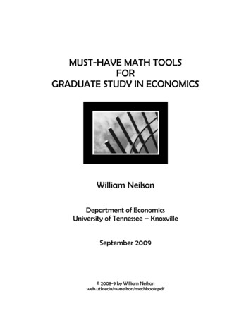
CHAPTER 2. SINGLE VARIABLE OPTIMIZATION9 π(q)qFigure 2.2: A pro t function with a minimumdecreasing q below q also reduces pro t. Second, the pro t function risesup to q and then falls. To see why this is important, compare it to Figure2.2, where the pro t function has a minimum. In Figure 2.2 the pro tfunction falls to the minimum then rises, while in Figure 2.1 it rises to themaximum then falls. To make sure we have a maximum, we have to makesure that the pro t function is rising then falling.This leaves us with several tasks. (1) We must nd the slope of the pro tfunction. (2) We must nd q by nding where the slope is zero. (3) Wemust make sure that pro t really is maximized at q , and not minimized.(4) We must relate our ndings back to economics.2.2DerivativesThe derivative of a function provides its slope at a point. It can be denotedin two ways: f 0 (x) or df (x) dx. The derivative of the function f at x isde ned asf (x h) f (x)df (x) lim:(2.1)h!0dxhThe idea is as follows, with the help of Figure 2.3. Suppose we start at xand consider a change to x h. Then f changes from f (x) to f (x h).The ratio of the change in f to the change in x is a measure of the slope:
CHAPTER 2. SINGLE VARIABLE OPTIMIZATION10f(x)f(x)f(x h)f(x)xxx hFigure 2.3: Approximating the slope of a function[f (x h) f (x)] [(x h) x]. Make the change in x smaller and smaller toget a more precise measure of the slope, and, in the limit, you end up withthe derivative.Finding the derivative comes from applying the formula in equation (2.1).And it helps to have a few simple rules in hand. We present these rules asa series of theorems.Theorem 1 Suppose f (x) a. Then f 0 (x) 0.Proof.f (x h)h!0ha a limh!0h 0:f 0 (x) limf (x)Graphically, a constant function, that is, one that yields the same value forevery possible x, is just a horizontal line, and horizontal lines have slopes ofzero. The theorem says that the derivative of a constant function is zero.Theorem 2 Suppose f (x) x. Then f 0 (x) 1.
CHAPTER 2. SINGLE VARIABLE OPTIMIZATION11Proof.f (x h) f (x)h!0h(x h) x limh!0hh limh!0 h 1:f 0 (x) limGraphically, the function f (x) x is just a 45-degree line, and the slope ofthe 45-degree line is one. The theorem con rms that the derivative of thisfunction is one.Theorem 3 Suppose f (x) au(x). Then f 0 (x) au0 (x).Proof.f (x h) f (x)h!0hau(x h) au(x) limh!0hu(x h) u(x) a limh!0h0 au (x):f 0 (x) limThis theorem provides a useful rule. When you multiply a function by ascalar (or constant), you also multiply the derivative by the same scalar.Graphically, multiplying by a scalar rotates the curve.Theorem 4 Suppose f (x) u(x) v(x). Then f 0 (x) u0 (x) v 0 (x).Proof.f (x h) f (x)h!0h[u(x h) v(x h)] [u(x) v(x)] limh!0hu(x h) u(x) v(x h) u(x) lim h!0hh00 u (x) v (x):f 0 (x) lim
CHAPTER 2. SINGLE VARIABLE OPTIMIZATION12This rule says that the derivative of a sum is the sum of the derivatives.The next theorem is the product rule, which tells how to take thederivative of the product of two functions.Theorem 5 Suppose f (x) u(x) v(x). Then f 0 (x) u0 (x)v(x) u(x)v 0 (x).Proof.f (x h) f (x)h[u(x h)v(x h)] [u(x)v(x)] limh!0h[u(x h) u(x)]v(x) u(x h)[v(x h) limh!0hhf 0 (x) limh!0v(x)]where the move from line 2 to line 3 entails adding then subtracting limh!0 u(x h)v(x) h. Remembering that the limit of a product is the product of thelimits, the above expression reduces to[u(x h) u(x)][v(x h)v(x) lim u(x h)h!0h!0hh00 u (x)v(x) u(x)v (x):f 0 (x) limv(x)]We need a rule for functions of the form f (x) 1 u(x), and it is providedin the next theorem.Theorem 6 Suppose f (x) 1 u(x). Then f 0 (x) u0 (x) [u(x)]2 .Proof.f (x h)h!0hf 0 (x) lim lim1u(x h)f (x)1u(x)hu(x) u(x h) limh!0 h[u(x h)u(x)][u(x h) u(x)]1 limlimh!0h!0 u(x h)u(x)h1 u0 (x):[u(x)]2h!0
CHAPTER 2. SINGLE VARIABLE OPTIMIZATION13Our nal rule concerns composite functions, that is, functions of functions.This rule is called the chain rule.Theorem 7 Suppose f (x) u(v(x)). Then f 0 (x) u0 (v(x)) v 0 (x).Proof. First suppose that there is some sequence h1 ; h2 ; ::: with limi!1 hi 0 and v(x hi ) v(x) 6 0 for all i. Thenf (x h) f (x)h!0hu(v(x h)) u(v(x))limh!0hu(v(x h)) u(v(x)) v(x h) v(x)limh!0v(x h) v(x)hu(v(x) k)) u(v(x))v(x h) v(x)limlimk!0h!0kh00u (v(x)) v (x):f 0 (x) lim Now suppose that there is no sequence as de ned above. Then there existsa sequence h1 ; h2 ; ::: with limi!1 hi 0 and v(x hi ) v(x) 0 for all i.Let b v(x) for all x,andf (x h) f (x)h!0hu(v(x h)) u(v(x)) limh!0hu(b) u(b) limh!0h 0:f 0 (x) limBut u0 (v(x)) v 0 (x) 0 since v 0 (x) 0, and we are done.Combining these rules leads to the following really helpful rule:da[f (x)]n an[f (x)]n 1 f 0 (x):dx(2.2)
CHAPTER 2. SINGLE VARIABLE OPTIMIZATION14This holds even if n is negative, and even if n is not an integer. So, forexample, the derivative of xn is nxn 1 , and the derivative of (2x 1)5 is10(2x 1)4 . The derivative of (4x2 1) :4 is :4(4x2 1) 1:4 (8x).Combining the rules also gives us the familiar division rule:u0 (x)v(x) v 0 (x)u(x)d u(x): dx v(x)[v(x)]2(2.3)To get it, rewrite u(x) v(x) as u(x) [v(x)] 1 . We can then use the productrule and expression (2.2) to getdu(x)v 1 (x)dx u0 (x)v 1 (x) ( 1)u(x)v 2 (x)v 0 (x)u0 (x) v(x)v 0 (x)u(x):v 2 (x)Multiplying both the numerator and denominator of the rst term by v(x)yields (2.3).Getting more ridiculously complicated, considerf (x) (x3 2x)(4xx31):To di erentiate this thing, split f into three component functions, f1 (x) x3 2x, f2 (x) 4x 1, and f3 (x) x3 . Then f (x) f1 (x) f2 (x) f3 (x),andf10 (x)f2 (x) f1 (x)f20 (x) f1 (x)f2 (x)f30 (x)0f (x) :f3 (x)f3 (x)[f3 (x)]2We can di erentiate the component functions to get f1 (x) 3x2 2, f20 (x) 4, and f30 (x) 3x2 . Plugging this all into the formula above gives us(3x2 2)(4xf (x) x302.31)4(x3 2x) x33(x3 2x)(4xx61)x2:Uses of derivativesIn economics there are three major uses of derivatives.The rst use comes from the economics idea of "marginal this" and "marginal that." In principles of economics courses, for example, marginal cost is
CHAPTER 2. SINGLE VARIABLE OPTIMIZATION15de ned as the additional cost a rm incurs when it produces one more unitof output. If the cost function is C(q), where q is quantity, marginal cost isC(q 1) C(q). We could divide output up into smaller units, though, bymeasuring in grams instead of kilograms, for example. Continually dividing output into smaller and smaller units of size h leads to the de nition ofmarginal cost asc(q h) c(q):M C(q) limh!0hMarginal cost is simply the derivative of the cost function. Similarly, marginal revenue is the derivative of the revenue function, and so on.The second use of derivatives comes from looking at their signs (the astrology of derivatives). Consider the function y f (x). We might askwhether an increase in x leads to an increase in y or a decrease in y. Thederivative f 0 (x) measures the change in y when x changes, and so if f 0 (x) 0we know that y increases when x increases, and if f 0 (x) 0 we know that ydecreases when x increases. So, for example, if the marginal cost functionM C(q) or, equivalently, C 0 (q) is positive we know that an increase in outputleads to an increase in cost.The third use of derivatives is for nding maxima and minima of functions.This is where we started the chapter, with a competitive rm choosing outputto maximize pro t. The pro t function is (q) R(q) C(q). As we saw inFigure 2.1, pro t is maximized when the slope of the pro t function is zero,ord 0:dqThis condition is called a rst-order condition, often abbreviated as FOC.Using our rules for di erentiation, we can rewrite the FOC asd R0 (q )dqC 0 (q ) 0;(2.4)which reduces to the familiar rule that a rm maximizes pro t by producingwhere marginal revenue equals marginal cost.Notice what we have done here. We have not used numbers or speci cfunctions and, aside from homework exercises, we rarely will. Using generalfunctions leads to expressions involving general functions, and we want tointerpret these. We know that R0 (q) is marginal revenue and C 0 (q) is marginal cost. We end up in the same place we do using graphs, which is a good
CHAPTER 2. SINGLE VARIABLE OPTIMIZATION16thing. The power of the mathematical approach is that it allows us to applythe same techniques in situations where graphs will not work.2.4Maximum or minimum?Figure 2.1 shows a pro t function with a maximum, but Figure 2.2 showsone with a minimum. Both of them generate the same rst-order condition:d dq 0. So what property of the function tells us that we are getting amaximum and not a minimum?In Figure 2.1 the slope of the curve decreases as q increases, while inFigure 2.2 the slope of the curve increases as q increases. Since slopes arejust derivatives of the function, we can express these conditions mathematically by taking derivatives of derivatives, or second derivatives. The secondderivative of the function f (x) is denoted f 00 (x) or d2 f dx2 . For the functionto have a maximum, like in Figure 2.1, the derivative should be decreasing,which means that the second derivative should be negative. For the functionto have a minimum, like in Figure 2.2, the derivative should be increasing,which means that the second derivative should be positive. Each of these iscalled a second-order condition or SOC. The second-order condition fora maximum is f 00 (x) 0, and the second-order condition for a minimum isf 00 (x) 0.We can guarantee that pro t is maximized, at least locally, if 00 (q ) 0.We can guarantee that pro t is maximized globally if 00 (q) 0 for all possiblevalues of q. Let’s look at the condition a little more closely. The rstderivative of the pro t function is 0 (q) R0 (q) C 0 (q) and the secondderivative is 00 (q) R00 (q) C 00 (q). The second-order condition for amaximum is 00 (q)0, which holds if R00 (q)0 and C 00 (q)0. So,we can guarantee that pro t is maximized if the second derivative of therevenue function is nonpositive and the second derivative of the cost functionis nonnegative. Remembering that C 0 (q) is marginal cost, the conditionC 00 (q) 0 means that marginal cost is increasing, and this has an economicinterpretation: each additional unit of output adds more to total cost thanany unit preceding it. The condition R00 (q) 0 means that marginal revenueis decreasing, which means that the rm earns less from each additional unitit sells.One special case that receives considerable attention in economics is theone in which R(q) pq, w
speak mathematics as a second language, that is, to make you comfortable talking about economics using the shorthand of mathematics. In undergrad-uate courses economic arguments are often made using graphs. In graduate courses we tend to use equations. But equ