Transcription
American Journal of Business Education – Third Quarter 2017Volume 10, Number 3NPV Sensitivity Analysis:A Dynamic Excel ApproachGeorge A. Mangiero, Iona College, USAMichael Kraten, Providence College, USAABSTRACTFinancial analysts generally create static formulas for the computation of NPV. When they do so, however, it is notreadily apparent how sensitive the value of NPV is to changes in multiple interdependent and interrelated variables.It is the aim of this paper to analyze this variability by employing a dynamic, visually graphic presentation usingExcel. Our approach illustrates how these variables, when increased or decreased to reflect the potential range ofvalues in a business case, change the value of NPV, and hence affect the decision about whether to proceed with theproject or to reject it.Furthermore, since sales revenue is one of the least certain elements in the business case, the presentation includesa probability estimate of whether NPV will be positive or negative, assuming that sales revenue is normallydistributed with a known mean and standard deviation.The business case we have chosen for illustrative purposes is a global energy project. Nevertheless, financialanalysts in any industry should be able to apply our dynamic spreadsheet approach to their projects as well.Keywords: Dynamic Forecasting; Financial Modeling; Net Present Value; Sensitivity Analysis; PedagogicalApplicationI. INTRODUCTIONAt the heart of Corporate Finance is the decision about whether to invest in capital assets, either toexpand the corporation’s capacity to produce its existing products or to replace obsolete or wornequipment. This decision, referred to as the “Capital Budgeting” decision, entails the usequantitative techniques which, if valid and used properly, should result in “yes” or “no” decisions that increase thevalue of the firm, and hence shareholder wealth, or prevent the value of the firm from decreasing.In a typical Corporate Finance course, several such quantitative techniques are presented, discussed and compared.These include: Payback, Discounted Payback, Internal Rate of Return (IRR), Profitability Index (PI), and NetPresent Value (NPV). This last method, NPV, is considered by most to be the premier method. “NPV is king!” is aquote by the author of a widely used textbook.NPV, like IRR and PI, is a discounted cash flow method. If a project’s NPV is computed and results in a positivevalue (NPV 0), the project is then considered to be one that will, if pursued, result in an increase in shareholderwealth. If the computation of NPV results in a negative value (NPV 0), the project should be rejected.Several steps are involved in the computation of NPV, including a determination of all of the risky and “riskless”incremental cash flows that result from initiation to completion of the project, determining an appropriate rate to usein the discounting process, and then applying the NPV formula to determine its value. Essentially, the methodcompares the present value of the project’s incremental benefits to the present value of its incremental costs. Manyvariables are involved in this process, including incremental revenues, incremental variable and fixed costs,incremental depreciation expense, the firm’s tax rate, and the relative uncertainty of the project’s cash flows, themarket and book values of existing equipment to be replaced and new equipment to be purchased at the beginningCopyright by author(s); CC-BY113The Clute Institute
American Journal of Business Education – Third Quarter 2017Volume 10, Number 3and end of the project, to name several of the more important. The relative uncertainty of the project’s cash flowscan be used to determine a risk-adjusted discount rate or to calculate certainty equivalent cash flows.Each of the factors that influence the NPV calculation represents an estimate. Some estimates can be establishedwith a significant degree of precision, but other estimates can only be established within a relatively broad range.When the level of uncertainty is relatively high, the range of the estimate is comparatively broad, and NPV can onlybe quantified with a limited degree of certainty.By simply creating a static formula for the computation of NPV, it is not readily apparent how sensitive the value ofNPV is to changes in these variables. Thus, it is the aim of this paper to analyze this sensitivity by using a dynamic(as opposed to a static*), visually graphic presentation using Excel. The resulting presentation illustrates how thevariables discussed above, when increased or decreased, change the value of NPV, and hence affect the decisionabout whether to proceed with the project or to reject it.Furthermore, since sales revenue is one of the least certain elements in the calculation, the presentation includes aprobability estimate of whether NPV will be positive or negative, assuming that sales revenue is normallydistributed with a known mean and standard deviation.* We have seen static approaches, used by accounting firms, which, though they are robust, are not aspedagogically illustrative as our dynamic approach. Our method emphasizes a vivid visual depiction of the impactof uncertainty produced by variations in projection variables on NPV.II. NPV CALCULATIONA. The static calculation of NPV is as follows:N CF0 CF1/ (1 k) 1 CF2/ (1 k) 2 CFN/ (1 k) Ni 0Each of these cash flows, except for CF0, occurs in the future and, hence, subject to uncertainty in terms of bothtiming and value.B. The benefits of a Dynamic Approach The analyst must be able to manipulate independent variables (singly or together) to quickly performsensitivity assessments. In the real world, such variables are often interrelated and independent,thereby making a static approach insufficient.The analyst must be concerned about the projects potential for breakeven at the same time as itspotential for surpassing minimum profitability requirements. Thus the analyst must utilize aspreadsheet tool that enables the simultaneous determination of several breakeven values. (Δ TR isused to illustrate this point in our case)This approach saves time in a pedagogical setting and makes the presentation more visually moreinteresting to students.III. A VISUALLY DYNAMIC ANALYTICAL APPROACH FOR QUANTIFYING UNCERTAINTYThe purpose of this section is to show visually how several features in Excel can be used to dynamicallydemonstrate to students how various independent variables affect NPV, or to put it another way, how sensitive NPVis to the various variables in the NPV equation. This is by no means an exhaustive inventory of the features orvariables available to the instructor for manipulation. This presentation is meant simply to show, with a fewexamples, what can be done and to suggest expansions in other directions.Copyright by author(s); CC-BY114The Clute Institute
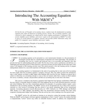
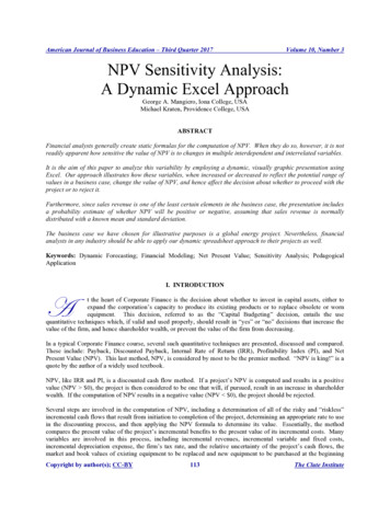
American Journal of Business Education – Third Quarter 2017Volume 10, Number 3We have chosen four key variables to manipulate using “spinners” available in Excel: Total Revenue (ΔTR),Variable Cost Ratio (VCR), Terminal Market Value (MV), and cost of capital (k). The initial investment, ΔTFC,ΔDEP, and the tax rate, T, are kept constant throughout (and thus have not been programmed with spinners) at 5,000,000, 6,000,000, 1,000,000, and 40% respectively.Our baseline variable values (See Figure 1), for this presentation were arbitrarily selected to be:ΔTR 6,500,000VCR 0.15MV 5,000,000k 5%For these values, NPV - 2,151,531.68 and IRR is -6.88%.The spinner attached to ΔTR, changes ΔTR in increments of 100,000.Keeping VCR, MV, and k at their baseline levels, we now manipulate ΔTR.In Figure 2, using the spinner, ΔTR is reduced 5,800,000.Consequently NPV declines to - 3,697,154.84 and IRR falls to -15.80%.In Figure 3, using the spinner, ΔTR is increased 7,200,000.NPV increases to - 605,908.51 and IRR rises to -1.71%.Notice that the ΔTRBE is 7,474,410.97. Increasing ΔTR to a value above this amount produces a positive NPV.Returning to the baseline values listed above, we now manipulate VCR.The spinner attached to VCR, changes VCR in increments of 0.01, or 1 percent.In Figure 4, using the spinner, VCR is increased to 0.25.NPV declines to - 3,840,027.59 and IRR falls to -16.64%.Notice that Δ TRBE is now 8,470,999.10, a value required to compensate for the higher VCR.In Figure 5, using the spinner, VCR is increased even further to 0.35.NPV declines to - 5,528,523.49 and IRR falls to -26.90%.Δ TRBE now rises to 9,774,229.73.In Figure 6, using the spinner, VCR is decreased to 0.05.NPV increases to - 463,035.78, IRR rises to 2.49%, and Δ TRBE falls to 6,687,630.87.Returning again to the baseline values listed above, we now manipulate MV.The spinner attached to MV, changes MV in increments of 250,000.In Figure 7, using the spinner, MV is increased to 10,000,000.As expected, NPV increases to 199,046.82 and IRR rises to 5.86%.Δ TRBE now falls to 6,409,853.34, as expected, in comparison to the baseline Δ TRBE.Returning one last time to the baseline values listed above, we now manipulate k.The spinner attached to k, changes k in increments of 1 percent.In Figure 8, using the spinner, k is decreased to 1.00%.In comparison to the baseline NPV, NPV increases to - 1,587,468.34 and IRR remains at -6.88%, since IRR is notaffected by changes in k.Δ TRBE falls to 7,141,332.55 in comparison to the baseline Δ TRBE, as a result of the lower k value.Copyright by author(s); CC-BY115The Clute Institute
American Journal of Business Education – Third Quarter 2017Volume 10, Number 3Note again that in these last five figures, ΔTRBE adjusts accordingly to account for the change in VCR, MV, and k –a valuable pedagogical point to make in a classroom setting. In other words, it is important to simultaneouslyconsider a myriad of concepts, factors, and variables (i.e., the breakeven concept, revenue elasticity concept, andaccounting estimates of various expenses) in a dynamic fashion by addressing all of these considerations in a singleΔTRBE metric.Statistical analysis can be added to the discussion by superimposing a distribution of one (any) of the variable on theplot. We chose ΔTR and assumed a normal distribution.Returning to the baseline values listed above, the distribution ON/OFF “switch” is set to the ON position and anormal distribution plot of Δ TR appears on the display. Spinners attached to µ(ΔTR) and σ(ΔTR) are used tochange the mean and standard deviation of the distribution. In Figures 9, 10, 11, an 12, the baseline values are keptas in figure 1 and four different combinations of µ(Δ TR) and σ(ΔTR) are illustrated. For example, in Figure 9, ifΔTR were normally distributed with a mean µ(ΔTR) 7,500,000 and a standard deviation σ(ΔTR) 400,000,then the probability of a negative NPV would be 47.45%, as shown. This is exactly equivalent to the probabilitythat ΔTR will be less than ΔTRBE 7,474,410.97, which is the area under the curve to the left of the ΔTRBE 7,474,410.97. This same discussion applies to Figures 10-12.IV. CASE APPLICATION: SAVE THE BLUE FROGOur Excel application has been adopted for use in the online case Save The Blue Frog (seewww.savethebluefrog.com). This learning activity is an integrated accounting case involving valuation,sustainability, controls and risk, and ethics.Save The Blue Frog was developed as an integrated application of social presence theory, cognitive complexitytheory, and gaming theory. Accordingly, it earned the Best Research Paper Award at the Strategic and EmergingTechnologies Workshop of the 2014 Annual Meeting of the American Accounting Association in Atlanta, Georgia.The case is designed to inculcate the principles of the scientific method and critical thinking by requiring the studentto proceed through a series of four modules. The first module establishes a traditional baseline valuation for a globalenergy project, and each of the subsequent three modules forces a reconsideration of the baseline projectionsbecause of future uncertainties involving an environmental threat to an endangered species, a litigation riskinvolving illicit payments, and a concern involving professional ethics.There are four features of the case that collectively require a visually dynamic approach to project analysis:1.2.3.4.The primary variables that impact the earnings and cash flow financial projections also impact eachother. Furthermore, the internal controls and other prospective solutions that are designed to addressthese variables likewise impact each other.Some of the variables are quantitative in nature, whereas others are qualitative in nature. Some wieldshort term effects on earnings and cash flows, whereas others wield long term effects. Some arepredictable, whereas others are unpredictable, and some are controllable, whereas others areuncontrollable.The baseline valuation illustrates a project that is cash flow solvent throughout its twenty year forecast,and yet falls just shy of an organization's target valuation metrics. It is thus necessary to considervarious modest-to-moderate modifications of the firm’s operating plans and expectations in order toassess the probability that the valuation targets may yet be achieved.The case is designed as a role playing activity that concludes with the development of a written reportand corresponding presentation. The goal of these tasks is to persuade the senior partner of a globalaccounting firm to accept the student's recommendations.These four features all emphasize the need for an analytical approach that can: (1) simultaneously assess the impactof different metrics in an extremely diverse collection of variables on the valuation of a project, and (2) present theCopyright by author(s); CC-BY116The Clute Institute
American Journal of Business Education – Third Quarter 2017Volume 10, Number 3outcomes in a visually persuasive manner that is suitable for written reports and presentations. We have designedour Excel application to serve these needs.V. IMPLICATIONSThe applications of our spreadsheet based analytical tool extend far beyond the development of visually dynamicpresentations of Net Present Value and other valuation metrics. The tool can also be utilized to assist managers inmaking critical decisions about a project’s continuing operations.Whereas Figures 1 through 8 illustrate how the tool’s forecasting function can be utilized to approve or reject initialproject investments, Figures 9 through 14 address the backcasting function for projects that are in the operationsstage. As year after year of actual operating TR data are accumulated, the mean and standard deviation of the actualdata will inevitably vary from the initial annual TR forecast.Thus, the spreadsheet tool’s P (NPV 0) metric represents a Key Performance Indicator (KPI) that can helpmanagers decide whether a series of disappointingly low actual TR outcomes should compel the suspension ortermination of operations. If this KPI exceeds a pre-established tolerance level, such a decision may be necessary.By adding statistical synopses of actual data to a spreadsheet that initially contained (and that continues to contain)projected estimates, financial analysts can effectively supplement their initial forecasting activities with subsequentbackcasting activities. After all, an intolerably high KPI may not solely be attributable to unforeseen events andcircumstances. It may also (or alternatively) be attributable to a badly flawed initial forecast.Figures 9 through 12 illustrate different applications of this KPI data function. Figures 13 and 14 then proceed todemonstrate how managers can utilize the spreadsheet tool to help monitor the strength of any particular projectwithin a broader portfolio of projects.Just as managers need to establish tolerance limits for the P (NPV 0) metric, they need to establish tolerance limitsfor other operating metrics as well. For instance, even though a project’s IRR may exceed the cost of capital,managers may require the project to produce an IRR that exceeds a minimum tolerance limit that is establishedabove the cost of capital.Why? Because, as a component of a portfolio, managers may need to rely on a project to produce sufficient free (orexcess) cash flows to finance the initial investment costs of future projects. Thus, even though a project’s IRR mayexceed its cost of capital, managers may still decide to reject it if its IRR falls below a level that can produce suchcash flows.Figures 13 and 14 illustrate such an analysis. By combining the portfolio managers' capabilities of these two Figureswith the backcasting capabilities of the preceding four Figures, managers can employ our dynamic spreadsheet toolin a manner that extends well beyond the initial determination of a project’s value.Indeed, the spreadsheet can continue to be utilized to assist in the ongoing oversight of the project’s operations. Forinstance, Figure 13 illustrates a value of ΔTR ( 7,500,000) that just exceeds ΔTRBE, and thus results in a positiveNPV. Figure 14 illustrates a value of ΔTR ( 7,600,000) that results in an IRR that exceeds the baseline IRR by 30percent.VI. CONCLUSIONThe initial investment, in the web based internet services industry, is a highly variable assumption because it ishighly dependent on the nature of the corporation’s fundamental strategy and long term goals. For instance, a startup web based services firm would require relatively little upfront investment funds if it opts to rent server space. Onthe other hand, it would require significant investment funds if it opts to build and own its own server funds.Copyright by author(s); CC-BY117The Clute Institute
American Journal of Business Education – Third Quarter 2017Volume 10, Number 3Likewise, a project at an established firm that relies on the cloud based platforms of a different technology firmwould require relatively little investment. Conversely, a firm project that relies on a “build it yourself” softwareplatform would require significant investment funds.Thus, we see that industry factors may dramatically impact the choice of variables that may be subjected to different“spinner” values on the Excel spreadsheet. Nevertheless, this would be true of both start-up firms and establishedfirms, as both types of firms utilize the same fundamental NPV calculation.Furthermore, our spreadsheet has been designed in a manner that reflects the fundamental goals of a dashboardreport. Just as classic dashboard reports summarize all of the critical elements (on a single page) that managers mustreview in order to maintain full control over their diverse business units, our spreadsheet presents (on a singleworksheet) all of the critical variables that financial analysts must assess in order to fully understand the value oftheir projects.We have demonstrated how several of the factors that influence the NPV calculation in a dynamic presentation.Because many of these factors will encompass a significant degree of uncertainty, a static approach to analyzingmany of these variables will not suffice. Thus, it is the aim of this paper to analyze this sensitivity by using adynamic, visually graphic presentation using Excel.AUTHOR BIOGRAPHIESMichael Kraten, PhD, CPA is an Associate Professor of Accounting at Providence College. He has earned a Ph.D.in behavioral accounting from the University of Connecticut, a M.P.P.M. in public and private management fromYale University, and a B.B.A. in public accounting from Baruch College of the City University of New York. Hisresearch interests include integrated reporting, investment valuation techniques, risk management, and sustainability.George A. Mangiero, PhD is an Associate Professor of Finance and Economics at Iona College in NewRochelle, New York. Dr. Mangiero’s graduate degrees include an MS in Electrical Engineering from RensselaerPolytechnic Institute, an MBA in Finance from St. John’sUniversity, and an M.Phil and Ph.D. in Finance from NewYork University. His research interests are primarily in the Areas of Portfolio Management, Financial Futures,Options and Swaps, and Corporate Finance. He resides with his wife in Connecticut.Copyright by author(s); CC-BY118The Clute Institute
American Journal of Business Education – Third Quarter 2017Volume 10, Number 3Figure 1.Figure 2.Copyright by author(s); CC-BY119The Clute Institute
American Journal of Business Education – Third Quarter 2017Volume 10, Number 3Figure 3.Figure 4.Copyright by author(s); CC-BY120The Clute Institute
American Journal of Business Education – Third Quarter 2017Volume 10, Number 3Figure 5.Figure 6.Copyright by author(s); CC-BY121The Clute Institute
American Journal of Business Education – Third Quarter 2017Volume 10, Number 3Figure 7.Figure 8.Copyright by author(s); CC-BY122The Clute Institute
American Journal of Business Education – Third Quarter 2017Volume 10, Number 3Figure 9.Figure 10.Copyright by author(s); CC-BY123The Clute Institute
American Journal of Business Education – Third Quarter 2017Volume 10, Number 3Figure 11.Figure 12.Copyright by author(s); CC-BY124The Clute Institute
American Journal of Business Education – Third Quarter 2017Volume 10, Number 3Figure 13.Figure 14.Copyright by author(s); CC-BY125The Clute Institute
American Journal of Business Education – Third Quarter 2017Volume 10, Number 3NOTESCopyright by author(s); CC-BY126The Clute Institute
A Dynamic Excel Approach George A. Mangiero, Iona College, USA Michael Kraten, Providence College, USA ABSTRACT Financial analysts generally create static formulas for the computation of NPV. When they do so, however, it is not readily apparent how sensitive the value of NPV is to chang