WIXLIB

varies among asset classes; a description of the dataset andtraining methodology is also included. At the end, weoffer our conclusions and discuss extensions of our work.Downloaded from https://jfds.pm-research.com by guest on June 16, 2020. Copyright 2020 Pageant Media Ltd.LITERATURE REVIEWIn this section, we review some classical tradingstrategies and discuss how RL has been applied to thisfield. Fundamental analysis aims to measure the intrinsicvalue of a security by examining economic data so investors can compare the security’s current price with estimates to determine whether the security is undervaluedor overvalued. One of the established strategies is calledCAN-SLIM (O’Neil 2009), and it is based on a majorstudy of market winners from 1880 to 2009. A commoncriticism of fundamental analysis is that the entranceand exit timing of trades is not specified. Even whenmarkets move toward the estimated price, bad timingin entering trades could lead to huge drawdowns, andsuch moves in account values are often not bearable toinvestors, shaking them out of the markets. Technicalanalysis is in contrast to fundamental analysis, in whicha security’s historical price data are used to study pricepatterns. Technicians place trades based on a combination of indicators such as the relative strength index(RSI) and Bollinger bands. However, owing to the lackof analysis on economic or market conditions, the predictability of these signals is not strong, often leadingto false breakouts.A lgorithmic trading is a more systematicapproach that involves mathematical modeling andautomated execution. Examples include trend following (Schwager 2017), mean-reversion (Chan 2013),statistical arbitrage (Chan 2009), and delta-neutraltrading strategies (Michaud 1989). We mainly reviewtime-series momentum strategies by Moskowitz,Ooi, and Pedersen (2012) because we benchmark ourmodels against their algorithms. Their work developeda very robust trading strategy by simply taking thesign of returns over the last year as a signal; they demonstrated profitability for every contract consideredwithin 58 liquid instruments over 25 years. Thenceforth, a number of methods (Baz et al. 2015; Baltasand Kosowski 2017; Rohrbach, Suremann, and Osterrieder 2017; Lim, Zohren, and Roberts 2019) have beenproposed to enhance this strategy by estimating thetrend and mapping to actual trade positions. However, these strategies are designed to profit from largeSpring 2020directional moves but can suffer huge losses if marketsmove sideways as the predictability of these signalsdeteriorates and excess turnover erodes profitability.Here, we adopt time-series momentum features alongwith technical indicators to represent state space andobtain trade positions directly using RL. The idea ofour representation is simple: extracting informationacross different momentum features and outputtingpositions based on the aggregated information.The current literature on RL in trading can becategorized into three main methods: critic-only, actoronly, and actor–critic approaches (Fischer 2018). Thecritic approach, mainly DQN, features most often inpublications in this field (Tan, Quek, and Cheng 2011;Bertoluzzo and Corazza 2012; Jin and El-Saawy 2016;Ritter 2017; Huang 2018). A state-action value function,Q, is constructed to represent how good a particularaction is in a state. Discrete action spaces are adoptedin these works, and an agent is trained to fully go longor short a position. However, a fully invested positionis risky during high-volatility periods, exposing oneto severe risk when opposite moves occur. Ideally, onewould like to scale positions up or down according tocurrent market conditions. Doing this requires one tohave large action spaces; however, the critic approachsuffers from large action spaces because a score must beassigned for each possible action.The second most common approach is the actoronly approach (Moody et al. 1998; Moody and Saffell2001; Deng et al. 2016; Lim, Zohren, and Roberts2019), in which the agent directly optimizes the objective function without computing the expected outcomesof each action in a state. Because a policy is directlylearned, actor-only approaches can be generalized tocontinuous action spaces. In the works of Moody andSaffell (2001) and Lim, Zohren, and Roberts (2019),off line batch gradient ascent methods can be used tooptimize the objective function, such as profits or Sharperatio, because the approach is differentiable end to end.However, this is different from standard RL actor-onlyapproaches in which a distribution needs to be learnedfor the policy. To study the distribution of a policy,the policy gradient theorem (Sutton and Barto 1998)and Monte Carlo methods (Metropolis and Ulam 1949)are adopted in the training, and models are updateduntil the end of each episode. We often experience slowlearning and need many samples to obtain an optimalpolicy because individual bad actions will be consideredThe Journal of Financial Data Science   3

Downloaded from https://jfds.pm-research.com by guest on June 16, 2020. Copyright 2020 Pageant Media Ltd.good as long as the total rewards are good; thus, a longtime is needed to adjust these actions.The actor–critic approach forms the third categoryand aims to solve the aforementioned learning problemsby updating the policy in real time. The key idea is toalternatively update two models in which one (the actor)controls how an agent performs given the current state,and the other (the critic) measures how good the chosenaction is. However, this approach is the least studiedmethod in financial applications (Li et al. 2007; Bekiros2010; Xiong et al. 2018). We aim to supplement theliterature and study the effectiveness of this approach intrading. For a more detailed discussion on state, actionspaces, and reward functions, interested readers arepointed to the survey (Fischer 2018). Other importantfinancial applications such as portfolio optimization andtrade execution are also included in this work.METHODOLOGYIn this section, we introduce our setups includingstate, action spaces, and reward functions. We describethree RL algorithms used in our work, DQN, PG, andA2C methods.We can formulate the trading problem as a Markovdecision process in which an agent interacts with theenvironment at discrete time steps. At each time step t, theagent receives some representations of the environmentdenoted as a state St. Given this state, an agent chooses anaction At, and based on this action, a numerical rewardRt 1 is given to the agent at the next time step, and theagent finds itself in a new state St 1. The interactionbetween the agent and the environment producesa trajectory τ [S 0, A 0, R 1, S 1, A1, R 2 , S 2 , A 2 , R 3, ].At any time step t, the goal of RL is to maximize theexpected return (essentially the expected discountedcumulative rewards) denoted as Gt at time t:T k t 1γ k t 1Rk(2)where g is the discounting factor. If the utility functionin Equation 1 has a linear form and we use Rt to represent trade returns, we can see that optimizing E(G) isequivalent to optimizing our expected wealth.4   Deep Reinforcement Learning for Trading Normalized close price series Returns over the past month, two months, threemonths, and one year are used. Following Lim,Zohren, and Roberts (2019), we normalize themby daily volatility adjusted to a reasonable timescale. As an example, we normalize annual returnsas rt 252,t /(σ t 252 ) , where σt is computed using anexponentially weighted moving standard deviationof rt with a 60-day span, MACD indicators are proposed by Baz et al. (2015)whereqtstd( qt 252:t )qt (m(S ) m(L ))/std( pt 63:t )MACDt Markov Decision Process FormalizationGt State space. In the literature, many differentfeatures have been used to represent state spaces.Among these features, a security’s past price is alwaysincluded, and the related technical indicators are oftenused (Fischer 2018). In our work, we take past price,returns (rt) over different horizons, and technical indicators including moving average convergence divergence(MACD) (Baz et al. 2015) and the RSI (Wilder 1978) torepresent states. At a given time step, we take the past 60observations of each feature to form a single state. Thefollowing is a list of our features:(3)where std(pt 63:t) is the 63-day rolling standarddeviation of prices pt , and m(S) is the exponentially weighted moving average of prices with atime scale S. The RSI is an oscillating indicator movingbetween 0 and 100. It indicates the oversold(a reading below 20) or overbought (above 80)condition of an asset by measuring the magnitudeof recent price changes. We include this indicatorwith a look-back window of 30 days in our staterepresentations.Action space. We study both discrete and continuous action spaces. For discrete action spaces, a simpleaction set of {-1, 0, 1} is used, and each value representsthe position directly (i.e., -1 corresponds to a maximallyshort position, 0 to no holdings, and 1 to a maximallylong position). This representation of action space is alsoknown as target orders (Huang 2018), in which a tradeposition is the output instead of the trading decision.Spring 2020

Downloaded from https://jfds.pm-research.com by guest on June 16, 2020. Copyright 2020 Pageant Media Ltd.Note that if the current action and next action are thesame, no transaction cost will occur and we just maintainour positions. If we move from a fully long position toa short position, transaction cost will be doubled. Thedesign of continuous action spaces is very similar to thediscrete case in which we still output trade positionsbut allow actions to be any value between -1 and 1(At [-1, 1]).Reward function. The design of the rewardfunction depends on the utility function in Equation 1.Here, we let the utility function be profits representinga risk-insensitive trader, and the reward Rt at time t isσ tgtσ tgtσ tgt Rt µ At 1rt bp pt 1 At 1 At 2 (4)σσσt 2t 1t 1 where stgt is the volatility target and st-1 is an exante volatility estimate calculated using an exponentially weighted moving standard deviation with a60-day window on rt. This expression forms the volatilityscaling of Moskowitz, Ooi, and Pedersen (2012), Harveyet al. (2018), and Lim, Zohren, and Roberts (2019), inwhich our position is scaled up when market volatility islow and vice versa. In addition, given a volatility target,our reward Rt is mostly driven by our actions instead ofbeing heavily affected by market volatility. We can alsoconsider the volatility scaling as normalizing rewardsfrom different contracts to the same scale. Because ourdataset consists of 50 futures contracts with differentprice ranges, we need to normalize different rewards tothe same scale for training and for portfolio construction. m is a fixed number per contract at each trade, andwe set it to 1. Note that our transaction cost term alsoincludes a price term pt 1. This is necessary because againwe work with many contracts, each of which has a different cost, so we represent transaction cost as a fractionof traded value. The constant, basis point (bp), is thecost rate and 1 bp 0.0001. As an example, if the costrate is 1 bp, we need to pay 0.10 to buy one unit of acontract priced at 1,000.We define rt pt - pt-1, and this expression represents additive profits. Additive profits are often used ifa fixed number of shares or contracts is traded at eachtime. If we want to trade a fraction of our accumulated wealth at each time, multiplicative profits shouldbe used, and rt pt pt-1 - 1. In this case, we also needto change the expression of R t because R t representsthe percentage of our wealth. The exact form is givenSpring 2020by Moody et al. (1998). We stick to additive profits inour work because logarithmic transformation needs tobe done for multiplicative profits to have the cumulative rewards required by the RL setup, but logarithmictransformation penalizes large wealth growth.RL AlgorithmsDQN. By adopting a neural network, a DQNapproximates the state-action value function (Q function) to estimate how good it is for the agent to performa given action in a given state. Suppose our Q functionis parameterized by some θ. We minimize the meansquared error between the current and target Q to derivethe optimal state-action value function:L (θ) E[(Qθ (S, A) Qθ′ (S, A))2 ]Qθ′ (St , At ) r γ argmax At 1Qθ (St 1 , At 1 )(5)where L(θ) is the objective function. A problem is thatthe training of a vanilla DQN is not stable and suffersfrom variability. Many improvements have been made tostabilize the training process, and we adopt the followingthree strategies to improve the training in our work:fixed Q-targets (Van Hasselt, Guez, and Silver 2016),double DQN (Hasselt 2010), and dueling DQN (Wanget al. 2016). Fixed Q-targets and double DQN are usedto reduce policy variances and to solve the problem ofchasing tails by using a separate network to produce targetvalues. Dueling DQNs separate the Q-value into statevalue and the advantage of each action. The benefit ofdoing this is that the value stream has more updates andwe receive a better representation of the state values.PG. The PG aims to maximize the expectedcumulative rewards by optimizing the policy directly.If we use a neural network with parameters θ to represent the policy, pθ(A S), we can generate a trajectoryτ [S 0, A 0, R 1, S1, , St , At , ] from the environmentand obtain a sequence of rewards. We maximize theexpected cumulative rewards J(θ) by using gradientascent to adjust θ: T 1 J (θ) E Rt 1 πθ t 0 T 1 θ J (θ) θ log πθ ( At St )Gt(6)t 0The Journal of Financial Data Science   5

Downloaded from https://jfds.pm-research.com by guest on June 16, 2020. Copyright 2020 Pageant Media Ltd.where G t is defined in Equation 2. Compared withDQN, PG learns a policy directly and can output a probability distribution over actions. This is useful if we wantto design stochastic policies or work with continuousaction spaces. However, the training of PG uses MonteCarlo methods to sample trajectories from the environment, and the update is done only when the episodefinishes. This often results in slow training, and it canget stuck at a (suboptimal) local maximum.A2C. The A2C is proposed to solve the trainingproblem of PG by updating the policy in real time. Itconsists of two models: One is an actor network thatoutputs the policy, and the other is a critic network thatmeasures how good the chosen action is in the givenstate. We can update the policy network p(A S, θ) bymaximizing the objective function:J (θ) E[log π( A S, θ)Aadv (S, A)](7)(8)To calculate advantages, we use another network,the critic network, with parameters w to model the statevalue function V (s w), and we can update the critic network using gradient descent to minimize the temporaldifference error:J (w ) ( Rt γV (St 1 w ) V (St w ))2(9)The A2C is most useful if we are interested incontinuous action spaces because we reduce the policyvariance by using the advantage function and update thepolicy in real time. The training of A2C can be donesynchronously or asynchronously (A3C). In this article,we adopt the synchronous approach and execute agentsin parallel on multiple environments.EXPERIMENTSDescription of DatasetWe use data on 50 ratio-adjusted continuousfutures contracts from the CLC Database (2019). Ourdataset ranges from 2005 to 2019 and consists of a varietyof asset classes, including commodity, equity index,fixed income, and FX. A full breakdown of the dataset6   Deep Reinforcement Learning for TradingBaseline AlgorithmsWe compare our methods to the following baseline models including classical time-series momentumstrategies: Long only Sign(R) (Moskowitz, Ooi, and Pedersen 2012; Lim,Zohren, and Roberts 2019):At sign(rt 252:t )(10) MACD signal (Baz et al. 2015)where Aadv(S, A) is the advantage function defined asAadv (St , At ) Rt γV (St 1 w ) V (St w )can be found in Appendix A. We retrain our model atevery five years, using all data available up to that pointto optimize the parameters. Model parameters are thenfixed for the next five years to produce out-of-sampleresults. In total, our testing period is from 2011 to 2019.At φ(MACDt )φ(MACD) MACD exp( MACD2 /4)0.89(11)where MACDt is defined in Equation 3. We canalso take multiple signals with different time scalesand average them to give a final indicator: t MACDt (Sk , L k )MACD(12)kwhere Sk and Lk define short and long time scales,namely Sk {8, 16, 32} and Lk {24, 48, 96}, asdone by Lim, Zohren, and Roberts (2019).We compare the aforementioned baseline modelswith our RL algorithms, DQN, PG, and A2C. DQNand PG have discrete action spaces {-1, 0, 1}, and A2Chas a continuous action space [-1, 1].Training Schemes for RLIn our work, we use long short-term memory(LSTM) (Hochreiter and Schmidhuber 1997) neural networks to model both actor and critic networks. LSTMsare traditionally used in natural language processing,but many recent works have applied them to financialtime series (Di Persio and Honchar 2016; Bao, Yue,Spring 2020

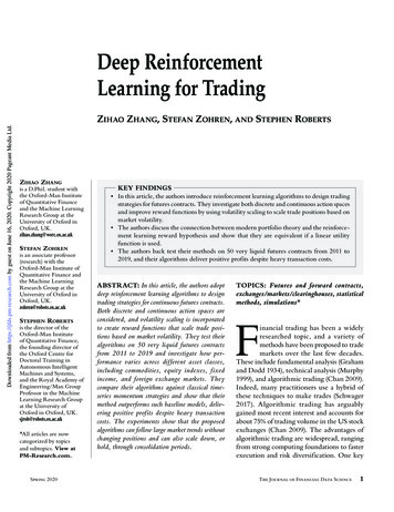
Exhibit 1Downloaded from https://jfds.pm-research.com by guest on June 16, 2020. Copyright 2020 Pageant Media Ltd.Values of Hyperparameters for Different RL Algorithms0RGHOαFULWLFαDFWRU2SWLPL]HU%DWFK 6L]HγES0HPRU\ 6L]Hτ'413* & GDP GDP GDP and Rao 2017; Tsantekidis et al. 2017b; Fischer andKrauss 2018). In particular, the work of Lim, Zohren,and Roberts (2019) showed that LSTMs deliver superiorperformance on modeling daily financial data. We usetwo-layer LSTM networks with 64 and 32 units in allmodels, and leaky rectifying linear units (Leaky-ReLU)(Maas, Hannun, and Ng 2013) are used as activationfunctions. Because our dataset consists of different assetclasses, we train a separate model for each asset class.It is a common practice to train models by groupingcontracts within the same asset class, and we find it alsoimproves our performance.We list the value of hyperparameters for differentRL algorithms in Exhibit 1. We denote the learningrates for critic and actor networks as acritic and aactor.The Adam optimizer (Kingma and Ba 2015) is usedfor training all networks, and batch size means the sizeof the minibatch used is in a gradient descent. As previously introduced, g is the discounting factor and bpis the cost rate used in training. We can treat bp as aregularizing term; a large bp penalizes turnovers and letsagents maintain current trade positions. The memorysize shows the size of the buffer for experience replay,and we update the parameters of our target network inDQN every t steps.Procedures for Controlling OverfittingBecause overfitting to backtest data can be problematic in many application domains, especially in finance,we adopt the following procedures to overcome it.The most common cause of overfitting is a poor ratio oftraining samples to model parameters. Although thereis no universal guarantee that increasing the number ofsamples will resolve the overfitting issue, we find thatexpanding the dataset to allow training on a cross section of futures contracts, not just on a single contract,greatly helps to reduce the problem in our case. Furthermore, we intentionally design our networks to have asmaller number of free parameters whenever possible.Spring 2020Our models consist of two hidden layers, and each layerhas a relatively small number of neurons. The resultingnetwork has fewer parameters, which makes it less likelyto overfit.In addition, we use dropout (Hinton et al. 2016),a regularization method commonly employed in deeplearning. Because our networks are small, we did notnotice significant improvements, but we still recommend the usage of dropout following the general adviceof selecting the least f lexible model that achieves comparable cross-validation performance. This is also in linewith other works (Zhang, Zohren, and Roberts 2018;Lim, Zohren, and Roberts 2019) that show improvedresults using dropout in financial applications, especiallywhen handling complex network architectures.Finally, we use 10% of any given training data asa separate cross-validation set to optimize hyperparameters. We monitor the validation performance and useearly stopping with 20 epochs to help optimal modelselection. Any hyperparameter optimization is done onthe cross-validation set, leaving the test set for the finaltest performance evaluation. This reduces the leakageof the test data, another cause of overfitting.Experimental ResultsWe test both baseline models and our methodsbetween 2011 and 2019, and we calculate the tradereturns net of transaction costs as in Equation 4 for eachcontract. We then form a simple portfolio by givingequal weights to each contract, and the trade return ofa portfolio isRtport 1 N i RtN i 1(13)where N represents the number of contracts considered,and Rti is the trade return for contract i at time t. Weevaluate the performance of this portfolio usingThe Journal of Financial Data Science   7

Downloaded from https://jfds.pm-research.com by guest on June 16, 2020. Copyright 2020 Pageant Media Ltd.following metrics as suggested by Lim, Zohren, andRoberts (2019):1. E(R): annualized expected trade returns2. std(R): annualized standard deviation of tradereturns3. Downside deviation (DD): annualized standarddeviation of trade returns that are negative, alsoknown as downside risk4. Sharpe: annualized Sharpe ratio (E(R) std(R))5. Sortino: a variant of the Sharpe ratio that usesdow

Deep Reinforcement Learning for Trading Spring 2020. component of such trading systems is a predictive signal that can lead to alpha (excess return); to this end, math-ematical and statistical methods are widely applied. However, because of the low signal-to-noise ratio