WIXLIB

system minimizes emotions throughout the trading process, ensures that discipline is maintainedthrough volatile market conditions, and allow us to achieve consistency.The other advantage of algorithmic trading over human traders is the ability to backtest thestrategy. Backtesting refers to applying a trading system to historical data to verify how a systemwould have performed during the specified time period. It helps the system developers learn howa trading strategy would performed in certain situations in the past, and is likely to perform in thefuture. It also provides the opportunity to optimize a trading strategy [26], by tweaking modelparameters over each iteration. The predictive power of backtesting rests on the importantassumption that the statistical properties of the price series are unchanging, so that the tradingrule that were profitable in the past will be profitable in the future [5]. However, such assumption issubject to invalidated risk, like changes in the macroeconomic prospect, fundamental of thecompany or structure of the financial market. Also, dividing historical data into in sample andout of sample sets during backtesting can provide traders a practical and efficient means forevaluating the system [13]. In sample data can be used to optimize the trading strategy, but it isimportant to then evaluate the system on clean out of sample data to determine its viability andeliminate overfitting.Moreover, an automated trading system can time the market well, which is extremely hardfor human investors. The legendary investor Warren Buffett has a famous quote: “We simplyattempt to be fearful when others are greedy and to be greedy only when others are fearful.” Thisis one form of an attempt to time the market when applying to every day trading. When people aregreedy, prices are overvalued thus a trader should sell the stock, and vice versa. But it isextremely hard to consistently identify when people are being greedy or fearful, as Buffett himselfalso said “our favorite holding period is forever”, which is a warning of do not try to time themarket. On the other hand, another form of timing the market is what High Frequency Tradingfirms does: find arbitrage opportunities and trade them within microseconds. At this frequency, it isimpossible for human to do so. However, automated trading systems can do a better job timingthe market, and even do so in a multi tasking way, which means that a system can time thousandsof stocks simultaneously. This is why HFT firms all use computerized trading algorithms, and withconsistent good financial time series forecasting, or sentiment analysis (analysing news articles ortweets), trading systems can also do a decent job at identifying greeds and fears in the market.7

2.3 Past ApproachesIn the domain of using machine learning techniques to forecast stock market movements,Financial Time Series Forecasting with Machine Learning Techniques: A Survey [17] provides acohesive overview of recent developments: Out of 46 publications this survey covers, 21 of themuse Artificial Neural Network based technology. 10 of them explore evolutionary or optimisationtechniques and the rest combine different algorithms into hybrid systems. 31 of them use a dailyfrequency, and 35 of them only use market index as the target. For evaluation methods, majorityof them use only forecast errors as the evaluation metric, and only three papers test their modelsin a real, or simulated trading environment, where one needs to concern with marginrequirements, trading cost and risk exposure.Stickel [31] tries to predict individual analyst’s forecast of corporate earning using thechange in the mean consensus forecast of other analysts. Huang [12] and Lu’s papers mainlyfocus on establishing Support Vector Machine models, or enhancing them with new trainingalgorithms to forecast major stock index. In particular, Lu [21] implements a regression model ofSVMs called Support Vector Regression, with the help of Vapnik’s epsilon insensitivity lossfunction. In The Performance of Several Combining Forecasts for Stock Index [34], Wang and Nieimplements a SVM based forecasts model, which combines the Grey model, BP neural networksand SVM, to predict the ShangHai Stock Index. Li [18] provides a different approach: he uses aNaive Bayesian machine learning approach to classify the information content of forward lookingstatements. He claims the Bayesian learning algorithm is better than a traditional dictionary basedapproach, in terms of the correlations between the predicted tones of forward looking statementsand current earnings.8

3. Machine Learning Methods3.1 Brief IntroductionAlan Turing, one of the greatest computer scientists in human history and father of artificialintelligence, in his paper “Computing Machinery and Intelligence” [33] asks this famous question:“Can machines think?” Until today, we as human still don’t know the answer to this question, butvariations of it has been answered. One of them is: Can machines learn? The answer is yes,supervised or unsupervised. And Machine Learning is the field of study which studies howmachines learn.According to Wikipedia, Machine Learning is a subfield of computer science that evolvedfrom the study of pattern recognition and computational learning theory in artificial intelligence [35].Arthur Samuel, a pioneer in artificial intelligence, defined machine learning as a “field of study thatgives computers the ability to learn without being explicitly programmed” [30]. Tom Mitchell, whoteaches at Carnegie Mellon University and is a prominent figure in the field of machine learning,defines it as “the study of computer algorithms that improve automatically through experience”[25]. In this book, Professor Mitchell provides a formal definition: A computer program is said tolearn from experience E with respect to some class of tasks T and performance measure P is itsperformance at tasks in T, as measured by P, improves with experience E [25].This interdisciplinary field has given birth and provided the theoretical foundation to the“Big Data” boom. One application of machine learning is “Data Mining”, which uses enormoushistorical data sets to improve decisions. Examples include turning medical records into medicalknowledge, or turning consumer transaction histories into targeting promotion advertisements.The other application is to develop softwares that we cannot program by hand, such asautonomous driving or speech recognition. Moreover, Deep Learning, which is again aninterdisciplinary field of machine learning and cognitive science, has made huge progress onimitating human brain activities. AlphaGo, which is the first computer program to beat a 9 danhuman world Go champion, is a product of deep learning techniques.There are many aspects of algorithmic trading, such as High Frequency Trading,Statistical Arbitrage and Financial Time Series Forecasting. In this paper, we focus on theforecasting realm, and examine what can machine learning algorithms achieve, not playing thegame of chess, but the game of forecasting stock prices.9

3.2 Basic Models & Variations3.2.1 Logistic RegressionLogistic regression was developed by statistician David Cox in his 1958 paper [8]. It is aspecial case of generalized linear model, and thus analogous to linear regression. The idea is toestimate the conditional probability of a binary response based on one or more predictor variablesby using the cumulative logistic distribution.If we have a binary output variable Y, and we want to model the conditional probabilityP(Y 1 X x) as a function of a vector x. Notice that log p(x) is a linear function of x, which has anunbounded range, but a easy modification, the logistic transformation log p/(1 p) is bounded.Therefore, the logistic regression model is(1)And solving for p, gives a form of the sigmoid function.(2)Figure 1: The logistic, or sigmoid, function.Two variations of logistic regression are implemented for the purpose of this paper.Logistic regression with a ridge penalty is used for the individual approach, and the lasso logistic10

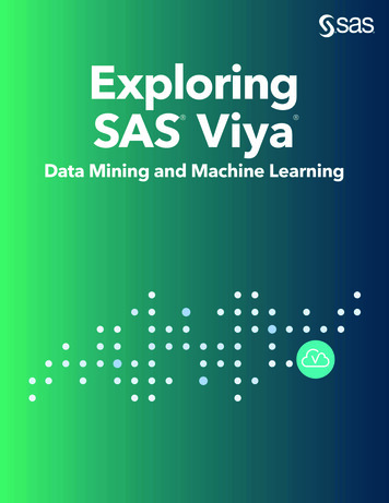
regression is used for the sector approach. The applications will be discussed in greater detaillater.Ridge regression minimizes(3)Where N is the number of observations, yi is the response at observation i, xi is the vectorof independent variables at observation i, βj are the coefficients of the original logistic regression,and lambda is the positive regularization parameter, also known as the ridge penalty. The secondterm shrinks the coefficients to prevent any one of the them being too large and cause overfitting.Similarly, the lasso regularization [32] minimizes(4)Instead of having the square term, the absolute value term is known as a L1 norm penalty.By increasing lambda, the lasso penalty also force the coefficients to shrink, but in this case theytend to be truncated at 0. Therefore, the lasso regularization can work as a feature selectionprocess.Figure 2: Example of the lasso logistic regression selecting meaningful coefficients11

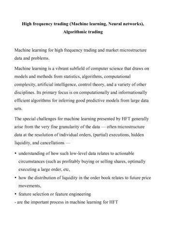
3.2.2 Decision TreeA decision tree is a hierarchical data structure implementing the divide and conquerstrategy, whereby the local region is identified in a sequence of recursive splits in a smallernumber of steps [1]. Therefore, a decision tree is composed of internal decision nodes andterminal leaves, see figure 3. Given an input, at each node, a test is applied and one of thebranches is taken depending on the outcome. This process starts at the root and is repeatedrecursively until a leaf node is hit, at which point the value written in the leaf constitutes the output.Figure 3: An example of a decision tree determining whether one can play outdoor sports based on weatherIn the case of a decision tree for classification, namely, a classification tree [4], thegoodness of a split is quantified by an impurity measure. One example of such measure is the Giniindex [4], which has the formula:(5)Where the sum is over the classes i at the node, and p(i) is the observed fraction ofclasses with class i that reach the node. A pure node, which is a node with just one class, has Giniindex 0, otherwise the Gini index is positive. If a node is not pure, then the instances should besplit again to decrease impurity, and there are multiple possible attributes on which we can split.Among all, we look for the split that minimizes impurity after the split because we want to generatethe smallest tree.12

However, a deep tree with many leaves still tends to overfit and therefore its test accuracyis often far less than its training accuracy. In contrast, a shallow tree can be more robust, that itstraining accuracy could be more close to that of a test set [3]. The decision tree model we use inthis paper is trimmed by minimize leaf size, that is, each leaf has at least a number of observationswe set, and more observations per leaf means less leaves and shallower tree.3.2.3 Naive BayesNaive Bayes classifiers are a family of simple probabilistic classifiers based on applyingBayes’ theorem with naive independence assumptions between the features. In other words, aNaive Bayes classifier assigns a new observation to the most probable class, assuming thefeatures are conditionally independent given the class value [25].The Naive Bayes classifier is,(6)Where vNB denotes the target value output by the Naive Bayes classifier, P(vj) is the prior,or class probability and the last term is the sample likelihood, which tess us how likely our sampleai is if the parameter of the distribution takes the value vj.Therefore, Naive Bayes classifies data in two steps: the training step, which uses thetraining data to estimate the parameters of a probability distribution, the prior probability and thesample likelihood. Then, the prediction step is, for any unseen test data, the method computes theposterior probability of that sample belonging to each class, and this data is classified as the classwith the largest posterior probability.In this paper, we pre assume that the data comes from a normal distribution, which makessense for stock returns [5] as they are generally randomly distributed with a mean of zero.Therefore, the Naive Bayes model estimates a separate normal distribution for each class bycomputing the mean and standard deviation of the training data in that class.Moreover, we use the ROC Curve analysis to optimize our Naive Bayes classifier. AReceiver Operating Characteristic (ROC) curve shows true positive rate versus false positive rate(equivalently, sensitivity versus 1 specificity) for different thresholds of the classifier output [23].13

Figure 4: An example of ROC curve and its optimal thresholdROC curve in general is used to compare performances across different classifiers, bycomparing each classifier’s AUC (area under curve) of its ROC curve. But in this case, we use theROC curve to find the threshold that maximizes the classification accuracy for the Naive Bayesclassifier. To do this, we find the slope S by:(7)Where Cost(N P) is the cost of misclassifying a positive class as a negative class, viceversa, and P TP FN and TN FP. The optimal operating point is found by moving the straightline with slope S from the upper left corner of the plot down and to the right, until it intersects withthe ROC curve, and the optimal threshold is the one associated with this operating point.3.2.4 Support Vector MachineSupport Vector Machine, which was introduced by Vapnik [7], maps the data into a higherdimensional input space and constructs an optimal separating, often linear hyperplane in thisspace. For separate classes, the optimal hyperplane maximizes a margin surrounding itself, whichcreates boundaries for the positive and negative classes, in a binary case. SVM imposes a penalty14

on the length of the margin for every observation that is on the wrong side of its class boundarywhen classes are inseparable.Figure 5: an example of a Support Vector Machine in a separable caseIn addition to performing linear classification, SVMs can efficiently perform a nonlinearclassification using the “kernel trick”, which implicitly maps the inputs into higher dimensionalfeature spaces. Without going into details, the SVM model in this paper uses the radial basiskernel, and the Matlab function automatically find an optimal scale value for the kernel function[24].3.3 Ensemble MethodsEach Machine learning algorithms we discussed above has many parameters to optimizefor and also many ways to perform the optimization. The “No Free Lunch” Theorem states that,there is no single learning algorithm that in any domain always induces the most accurate learner[38]. Also, each learning algorithm dictates a certain model that comes with a set of assumptions.This inductive bias leads to error if the assumptions do not hold for future data. In other words,learning is an ill posed problem, and with finite data, each algorithm converges to a differentsolution and fails under different circumstances [1]. Therefore, these problems raise the incentiveto explore models that composes of multiple base learners that complement each other bycombining them. The idea is that, there may always be another learner that is more accurate, and15

by suitably combining multiple base learners, overall accuracy can be improved. In general, thisapproach is called the Ensemble Method.We explore two ideas of ensemble method in this paper. The first one is Voting, which isthe simplest way to combine multiple classifiers.(8)Where wj is the weight of each base learner and dji is the classified output of each learnergiven a data point. In our case, all base learners are given equal weight, and the votes arecombined linearly by simply adding them up. The final decision is made based on the majority ofthe votes.The second ensemble takes the idea of the Random Subspace Method [11], whichrandomly chooses different input representations from the original data input, and then combinesclassifiers using different input features. This has the effect that different learners will look at thesame problem from different points of view and will be robust. It can also help reduce the curse ofdimensionality because each input data set is fewer dimensional.Other common ensemble methods that are not examined in this paper includesError Correcting Output Codes [9] (ECOC), Bagging, and Boosting [27].16

4. Prediction Model: Individual Approach4.1 MethodologyThe first method to develop a stock price prediction model is what we called an individualapproach, which means that the model uses historical performance of a stock itself to predict itsfuture price movements. The idea is that, looking at how the stock historically moves in N daywindows, there are patterns useful to predict the future price given a new N day window. Noticethat this approach ignores important factors such as general market information and performancesof competing companies, but we believe this simplified model can provide a good starting pointand a benchmark for comparison with complex models later.Some details about implementing this model needs to be addressed. First, we want tomake this a classification problem instead of a regression problem because we can use probabilitymodels like logistic regression to control the “confidence level” of the predictions and moreover, itis not necessary to predict the right price as long as we get the direction right. To see this, let’sassume a regression problem setting and suppose a stock with price 100 and 101 for today andtomorrow. Two models give different predictions of 99 and 110 for tomorrow. The first one isclose to the true price but it would suggest a sell and we lose money, while the second one,though has higher error, gets the right direction and we would profit from it. Second, we use dailyreturns instead of prices when building the dataset. Since most price series are geometric randomwalks, it violates the econometrics requirement that the expected value of error in a regressionneeds to be zero.but the returns are usually randomly distributed around a mean of zero [5].On top of logistic regression, we added a ridge penalty to prevent overfitting. A ridgepenalty can be used in logistic regression to improve the parameter estimates and to diminishout of sample error, by imposing a restriction on the parameters.By tweaking lambda we can restrict any one of the estimated coefficients to be too large.To see why this would help our model, suppose we want to predict tomorrow’s return by usingreturns from last seven days. The coefficient for yesterday’s return would be significantly largerthan the rest of them, because yesterday is the most relevant to today. However, one parameterbeing dominate significantly increase the chance to overfit, that is, the model would give too muchweight on yesterday while we want to consider the whole week. By applying the penalty, we canprevent this situation from happening and give more weights to the “further back” parameters.17

4.2 DataThe data we use is web scraped from Yahoo Finance, which contains adjusted closingprice for all the stocks in S&P 500 from Jan 2,2014 to Feb 1, 2016. We did not go further backbecause prices more than 2 years old is likely to be irrelevant. Adjusted closing price is the dailyclosing price, which is the last trading price before market closes at 4 pm, adjusted for dividendsand stock

The explosion of algorithmic trading, or automated trading system, has been one of the most prominent trends in the financial industry over recent decade. An automated trading system utilizes advanced quantitative models to generate certain