Transcription
Interactive Linear Algebra
Interactive Linear AlgebraDan MargalitGeorgia Institute of TechnologyJoseph RabinoffGeorgia Institute of TechnologyJune 3, 2019
2017Georgia Institute of TechnologyPermission is granted to copy, distribute and/or modify this document under theterms of the GNU Free Documentation License, Version 1.2 or any later versionpublished by the Free Software Foundation; with no Invariant Sections, no FrontCover Texts, and no Back-Cover Texts. A copy of the license is included in theappendix entitled “GNU Free Documentation License.” All trademarks are theregistered marks of their respective owners.
Contributors to this textbookDAN MARGALITSchool of MathematicsGeorgia Institute of Technologydmargalit7@math.gatech.eduLARRY ROLENSchool of MathematicsGeorgia Institute of Technologylarry.rolen@math.gatech.eduJOSEPH RABINOFFSchool of MathematicsGeorgia Institute of Technologyrabinoff@math.gatech.eduJoseph Rabinoff contributed all of the figures, the demos, and the technicalaspects of the project, as detailed below. The textbook is written in XML and compiled using a variant of RobertBeezer’s MathBook XML, as heavily modified by Rabinoff. The mathematical content of the textbook is written in LaTeX, then convertedto HTML-friendly SVG format using a collection of scripts called PreTeX: thiswas coded by Rabinoff and depends heavily on Inkscape for pdf decodingand FontForge for font embedding. The figures are written in PGF/TikZ andprocessed with PreTeX as well. The demonstrations are written in JavaScript WebGL using Steven Wittens’brilliant framework called MathBox.All source code can be found on GitHub. It may be freely copied, modified, andredistributed, as detailed in the appendix entitled “GNU Free Documentation License.”Larry Rolen wrote many of the exercises.v
vi
Variants of this textbookThere are several variants of this textbook available. The master version is the default version of the book. The version for math 1553 is fine-tuned to contain only the material coveredin Math 1553 at Georgia Tech.The section numbering is consistent across versions. This explains why Section6.3 does not exist in the Math 1553 version, for example.You are currently viewing the master version.vii
viii
OverviewThe Subject of This Textbook Before starting with the content of the text, wefirst ask the basic question: what is linear algebra? Linear: having to do with lines, planes, etc. Algebra: solving equations involving unknowns.The name of the textbook highlights an important theme: the synthesis betweenalgebra and geometry. It will be very important to us to understand systems oflinear equations both algebraically (writing equations for their solutions) and geometrically (drawing pictures and visualizing).Remark. The term “algebra” was coined by the 9th century mathematician AbuJa’far Muhammad ibn Musa al-Khwarizmi. It comes from the Arabic word al-jebr,meaning reunion of broken parts.At the simplest level, solving a system of linear equations is not very hard. Youprobably learned in high school how to solve a system like(x 3y z 42x y 3z 17y 4z 3.However, in real life one usually has to be more clever. Engineers need to solve many, many equations in many, many variables.Here is a tiny example: 3x 1 4x 2 7x 2x12 x 9x 2 1 1x 4x22 1 10x 3 13x 3 32 x 3 10x 3 19x 4 7x 4 x4 11x 4 2x 5 21x 5 14x 5 2x 5 3x 6 8x 6 27x 6 x6 141 2567 26 15. Often it is enough to know some information about the set of solutions,without having to solve the equations in the first place. For instance, doesthere exist a solution? What does the solution set look like geometrically?Is there still a solution if we change the 26 to a 27?ix
x Sometimes the coefficients also contain parameters, like the eigenvalue equation((7 λ)x y 3z 0 3x (2 λ) y 3z 0 3x 2 y ( 1 λ)z 0. In data modeling, a system of equations generally does not actually have asolution. In that case, what is the best approximate solution?Accordingly, this text is organized into three main sections.1. Solve the matrix equation Ax b (chapters 2–4). Solve systems of linear equations using matrices, row reduction, andinverses. Analyze systems of linear equations geometrically using the geometryof solution sets and linear transformations.2. Solve the matrix equation Ax λx (chapters 5–6). Solve eigenvalue problems using the characteristic polynomial. Understand the geometry of matrices using similarity, eigenvalues, diagonalization, and complex numbers.3. Approximately solve the matrix equation Ax b (chapter 7). Find best-fit solutions to systems of linear equations that have no actualsolution using least-squares approximations. Study the geometry of closest vectors and orthogonal projections.This text is roughly half computational and half conceptual in nature. Themain goal is to present a library of linear algebra tools, and more importantly, toteach a conceptual framework for understanding which tools should be applied ina given context.If Matlab can find the answer faster than you can, then your question is justan algorithm: this is not real problem solving.The subtle part of the subject lies in understanding what computation to askthe computer to do for you—it is far less important to know how to perform computations that a computer can do better than you anyway.
xiUses of Linear Algebra in Engineering The vast majority of undergraduates atGeorgia Tech have to take a course in linear algebra. There is a reason for this:Most engineering problems, no matter how complicated, can be reduced tolinear algebra:Ax borAx λxorAx b.Here we present some sample problems in science and engineering that requirelinear algebra to solve.Example (Civil Engineering). The following diagram represents traffic flow aroundthe town square. The streets are all one way, and the numbers and arrows indicate the number of cars per hour flowing along each street, as measured by sensorsunderneath the roads.Traffic flow (cars/hr)250120x12070yw175530z115390There are no sensors underneath some of the streets, so we do not know howmuch traffic is flowing around the square itself. What are the values of x, y, z, w?Since the number of cars entering each intersection has to equal the number ofcars leaving that intersection, we obtain a system of linear equations: w 120 x 250 x 120 y 70 y 530 z 390z 115 w 175.
xiiExample (Chemical Engineering). A certain chemical reaction (burning) takesethane and oxygen, and produces carbon dioxide and water:x C2 H6 y O2 z CO2 w H2 OWhat ratio of the molecules is needed to sustain the reaction? The followingthree equations come from the fact that the number of atoms of carbon, hydrogen, and oxygen on the left side has to equal the number of atoms on the right,respectively:2x z6x 2w2 y 2z w.Example (Biology). In a population of rabbits,1. half of the newborn rabbits survive their first year;2. of those, half survive their second year;3. the maximum life span is three years;4. rabbits produce 0, 6, 8 baby rabbits in their first, second, and third years,respectively.If you know the rabbit population in 2016 (in terms of the number of first, second, and third year rabbits), then what is the population in 2017? The rules forreproduction lead to the following system of equations, where x, y, z represent thenumber of newborn, first-year, and second-year rabbits, respectively: 6 y2016 8z2016 x 2017 1 y20172 x 20161 y z2017 .2 2016A common question is: what is the asymptotic behavior of this system? What willthe rabbit population look like in 100 years? This turns out to be an eigenvalueproblem.Use this link to view the online demoLeft: the population of rabbits in a given year. Right: the proportions of rabbits inthat year. Choose any values you like for the starting population, and click “Advance1 year” several times. What do you notice about the long-term behavior of the ratios?This phenomenon turns out to be due to eigenvectors.
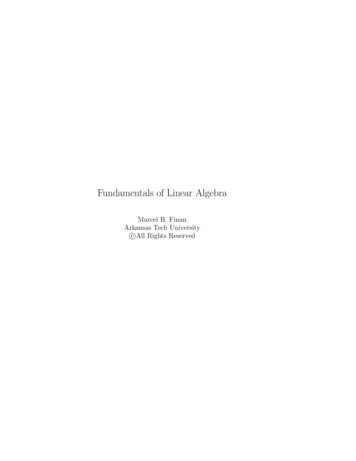
xiiiExample (Astronomy). An asteroid has been observed at the following locations:(0, 2), (2, 1), (1, 1), ( 1, 2), ( 3, 1), ( 1, 1).Its orbit around the sun is elliptical; it is described by an equation of the formx 2 B y 2 C x y Dx E y F 0.What is the most likely orbit of the asteroid, given that there was some significant error in measuring its position? Substituting the data points into the aboveequation yields the system(0)2(2)2(1)2( 1)2( 3)2( 1)2 B(2)2 B(1)2 B( 1)2 B( 2)2 B(1)2 B( 1)2 C(0)(2) D(0) E(2) C(2)(1) D(2) E(1) C(1)( 1) D(1) E( 1) C( 1)( 2) D( 1) E( 2) C( 3)(1) D( 3) E(1) C( 1)( 1) D( 1) E( 1) FFFFFF 000000.There is no actual solution to this system due to measurement error, but here isthe best-fitting ellipse:(0, 2)( 3, 1)( 1, 1)(2, 1)(1, 1)( 1, 2)266x 2 405 y 2 178x y 402x 123 y 1374 0Example (Computer Science). Each web page has some measure of importance,which it shares via outgoing links to other pages. This leads to zillions of equationsin zillions of variables. Larry Page and Sergei Brin realized that this is a linearalgebra problem at its core, and used the insight to found Google. We will discussthis example in detail in Section 5.6.
xivHow to Use This Textbook There are a number of different categories of ideasthat are contained in most sections. They are listed at the top of the section, underObjectives, for easy review. We classify them as follows. Recipes: these are algorithms that are generally straightforward (if sometimes tedious), and are usually done by computer in real life. They arenonetheless important to learn and to practice. Vocabulary words: forming a conceptual understanding of the subject of linear algebra means being able to communicate much more precisely than inordinary speech. The vocabulary words have precise definitions, which mustbe learned and used correctly. Essential vocabulary words: these vocabulary words are essential in that theyform the essence of the subject of linear algebra. For instance, if you do notknow the definition of an eigenvector, then by definition you cannot claimto understand linear algebra. Theorems: these describe in a precise way how the objects of interest relateto each other. Knowing which recipe to use in a given situation generallymeans recognizing which vocabulary words to use to describe the situation,and understanding which theorems apply to that problem. Pictures: visualizing the geometry underlying the algebra means interpretingand drawing pictures of the objects involved. The pictures are meant to bea core part of the material in the text: they are not just a pretty add-on.This textbook is exclusively targeted at Math 1553 at Georgia Tech. As such,it contains exactly the material that is taught in that class; no more, and no less:students in Math 1553 are responsible for understanding all visible content. In theonline version some extra material (most examples and proofs, for instance) ishidden, in that one needs to click on a link to reveal it, like this:Hidden Content. Hidden content is meant to enrich your understanding of thetopic, but is not an official part of Math 1553. That said, the text will be veryhard to follow without understanding the examples, and studying the proofs is anexcellent way to learn the conceptual part of the material. (Not applicable to thePDF version.)Finally, we remark that there are over 140 interactive demos contained in thetext, which were created to illustrate the geometry of the topic. Click the “view ina new window” link, and play around with them! You will need a modern browser.Internet Explorer is not a modern browser; try Safari, Chrome, or Firefox. Here isa demo from Section 6.5:Use this link to view the online demoClick and drag the points on the grid on the right.
xvFeedback Every page of the online version has a link on the bottom for providingfeedback. This will take you to the GitHub Issues page for this book. It requires aGeorgia Tech login to access.
xvi
ContentsContributors to this textbookvVariants of this textbookviiOverviewix1 Systems of Linear Equations: Algebra1.1 Systems of Linear Equations . . . . . . . . . . . . . . . . . . . . . . . .1.2 Row Reduction . . . . . . . . . . . . . . . . . . . . . . . . . . . . . . . . .1.3 Parametric Form . . . . . . . . . . . . . . . . . . . . . . . . . . . . . . . .1111242 Systems of Linear Equations: Geometry2.1 Vectors . . . . . . . . . . . . . . . . . . .2.2 Vector Equations and Spans . . . . . .2.3 Matrix Equations . . . . . . . . . . . .2.4 Solution Sets . . . . . . . . . . . . . . .2.5 Linear Independence . . . . . . . . . .2.6 Subspaces . . . . . . . . . . . . . . . . .2.7 Basis and Dimension . . . . . . . . . .2.8 Bases as Coordinate Systems . . . . .2.9 The Rank Theorem . . . . . . . . . . .3 Linear Transformations and Matrix Algebra3.1 Matrix Transformations . . . . . . . . . . .3.2 One-to-one and Onto Transformations . .3.3 Linear Transformations . . . . . . . . . . . .3.4 Matrix Multiplication . . . . . . . . . . . . .3.5 Matrix Inverses . . . . . . . . . . . . . . . .3.6 The Invertible Matrix Theorem . . . . . . .2930374453658192101108.1131141291411531681824 Determinants1874.1 Determinants: Definition . . . . . . . . . . . . . . . . . . . . . . . . . . 1874.2 Cofactor Expansions . . . . . . . . . . . . . . . . . . . . . . . . . . . . . 2064.3 Determinants and Volumes . . . . . . . . . . . . . . . . . . . . . . . . . 222xvii
xviii5 Eigenvalues and Eigenvectors5.1 Eigenvalues and Eigenvectors .5.2 The Characteristic Polynomial5.3 Similarity . . . . . . . . . . . . .5.4 Diagonalization . . . . . . . . .5.5 Complex Eigenvalues . . . . . .5.6 Stochastic Matrices . . . . . . .CONTENTS.6 Orthogonality6.1 Dot Products and Orthogonality6.2 Orthogonal Complements . . . .6.3 Orthogonal Projection . . . . . .6.4 Orthogonal Sets . . . . . . . . . .6.5 The Method of Least Squares . .237238252260277300322.339340347356373386A Complex Numbers409B Notation413C Hints and Solutions to Selected Exercises415D GNU Free Documentation License417Index427
Chapter 1Systems of Linear Equations:AlgebraPrimary Goal. Solve a system of linear equations algebraically in parametric form.This chapter is devoted to the algebraic study of systems of linear equationsand their solutions. We will learn a systematic way of solving equations of theform 3x 1 4x 2 10x 3 19x 4 2x 5 3x 6 141 7x 2x 13x 7x 21x 8x 25671234563 x 9x 2 2 x 3 x 4 14x 5 27x 6 26 1 1x 6 15.2 x 1 4x 2 10x 3 11x 4 2x 5 In Section 1.1, we will introduce systems of linear equations, the class of equations whose study forms the subject of linear algebra. In Section 1.2, will presenta procedure, called row reduction, for finding all solutions of a system of linearequations. In Section 1.3, you will see hnow to express all solutions of a systemof linear equations in a unique way using the parametric form of the general solution.1.1Systems of Linear EquationsObjectives1. Understand the definition of Rn , and what it means to use Rn to label pointson a geometric object.2. Pictures: solutions of systems of linear equations, parameterized solutionsets.3. Vocabulary words: consistent, inconsistent, solution set.1
2CHAPTER 1. SYSTEMS OF LINEAR EQUATIONS: ALGEBRADuring the first half of this textbook, we will be primarily concerned with understanding the solutions of systems of linear equations.Definition. An equation in the unknowns x, y, z, . . . is called linear if both sidesof the equation are a sum of (constant) multiples of x, y, z, . . ., plus an optionalconstant.For instance,3x 4 y 2z x z 100are linear equations, but3x yz 3sin(x) cos( y) 2are not.We will usually move the unknowns to the left side of the equation, and movethe constants to the right.A system of linear equations is a collection of several linear equations, like(x 2 y 3z 62x 3 y 2z 14(1.1.1)3x y z 2.Definition (Solution sets). A solution of a system of equations is a list of numbers x, y, z, . . . that makeall of the equations true simultaneously. The solution set of a system of equations is the collection of all solutions. Solving the system means finding all solutions with formulas involving somenumber of parameters.A system of linear equations need not have a solution. For example, there donot exist numbers x and y making the following two equations true simultaneously:§x 2y 3x 2 y 3.In this case, the solution set is empty. As this is a rather important property of asystem of equations, it has its own name.Definition. A system of equations is called inconsistent if it has no solutions. Itis called consistent otherwise.A solution of a system of equations in n variables is a list of n numbers. Forexample, (x, y, z) (1, 2, 3) is a solution of (1.1.1). As we will be studyingsolutions of systems of equations throughout this text, now is a good time to fixour notions regarding lists of numbers.
1.1. SYSTEMS OF LINEAR EQUATIONS1.1.13Line, Plane, Space, Etc.We use R to denote the set of all real numbers, i.e., the number line. This containsnumbers like 0, 32 , π, 104, . . .Definition. Let n be a positive whole number. We defineRn all ordered n-tuples of real numbers (x 1 , x 2 , x 3 , . . . , x n ).An n-tuple of real numbers is called a point of Rn .In other words, Rn is just the set of all (ordered) lists of n real numbers. Wewill draw pictures of Rn in a moment, but keep in mind that this is the definition.For example, (0, 23 , π) and (1, 2, 3) are points of R3 .Example (The number line). When n 1, we just get R back: R1 R. Geometrically, this is the number line. 3 2 10123Example (The Euclidean plane). When n 2, we can think of R2 as the x y-plane.We can do so because every point on the plane can be represented by an orderedpair of real numbers, namely, its x- and y-coordinates.(1, 2)(0, 3)
4CHAPTER 1. SYSTEMS OF LINEAR EQUATIONS: ALGEBRAExample (3-Space). When n 3, we can think of R3 as the space we (appearto) live in. We can do so because every point in space can be represented by anordered triple of real numebrs, namely, its x-, y-, and z-coordinates.(1, 1, 3)( 2, 2, 2)Interactive: Points in 3-Space.Use this link to view the online demoA point in 3-space, and its coordinates. Click and drag the point, or move the sliders.So what is R4 ? or R5 ? or Rn ? These are harder to visualize, so you have togo back to the definition: Rn is the set of all ordered n-tuples of real numbers(x 1 , x 2 , x 3 , . . . , x n ).They are still “geometric” spaces, in the sense that our intuition for R2 and R3often extends to Rn .We will make definitions and state theorems that apply to any Rn , but we willonly draw pictures for R2 and R3 .The power of using these spaces is the ability to label various objects of interest,such as geometric objects and solutions of systems of equations, by the points ofRn .Example (Color Space). All colors you can see can be described by three quantities: the amount of red, green, and blue light in that color. (Humans are trichromatic.) Therefore, we can use the points of R3 to label all colors: for instance, thepoint (.2, .4, .9) labels the color with 20% red, 40% green, and 90% blue intensity.
5blue1.1. SYSTEMS OF LINEAR EQUATIONSngreeredExample (Traffic Flow). In the Overview, we could have used R4 to label theamount of traffic (x, y, z, w) passing through four streets. In other words, if thereare 10, 5, 3, 11 cars per hour passing through roads x, y, z, w, respectively, thenthis can be recorded by the point (10, 5, 3, 11) in R4 . This is useful from a psychological standpoint: instead of having four numbers, we are now dealing with justone piece of data.xywzExample (QR Codes). A QR code is a method of storing data in a grid of blackand white squares in a way that computers can easily read. A typical QR codeis a 29 29 grid. Reading each line left-to-right and reading the lines top-tobottom (like you read a book) we can think of such a QR code as a sequence of29 29 841 digits, each digit being 1 (for white) or 0 (for black). In such away, the entire QR code can be regarded as a point in R841 . As in the previousexample, it is very useful from a psychological perspective to view a QR code as asingle piece of data in this way.
6CHAPTER 1. SYSTEMS OF LINEAR EQUATIONS: ALGEBRAThe QR code for this textbook is a 29 29 array of black/white squares.In the above examples, it was useful from a psychological perspective to replacea list of four numbers (representing traffic flow) or of 841 numbers (representing aQR code) by a single piece of data: a point in some Rn . This is a powerful concept;starting in Section 2.2, we will almost exclusively record solutions of systems oflinear equations in this way.1.1.2Pictures of Solution SetsBefore discussing how to solve a system of linear equations below, it is helpful tosee some pictures of what these solution sets look like geometrically.One Equation in Two Variables. Consider the linear equation x y 1. We canrewrite this as y 1 x, which defines a line in the plane: the slope is 1, andthe x-intercept is 1.Definition (Lines). For our purposes, a line is a ray that is straight and infinite inboth directions.
1.1. SYSTEMS OF LINEAR EQUATIONS7One Equation in Three Variables. Consider the linear equation x y z 1.This is the implicit equation for a plane in space.zyxDefinition (Planes). A plane is a flat sheet that is infinite in all directions.Remark. The equation x y z w 1 defines a “3-plane” in 4-space, andmore generally, a single linear equation in n variables defines an “(n 1)-plane”in n-space. We will make these statements precise in Section 2.7.Two Equations in Two Variables. Now consider the system of two linear equations§x 3 y 32x y 8.Each equation individually defines a line in the plane, pictured below.
8CHAPTER 1. SYSTEMS OF LINEAR EQUATIONS: ALGEBRAA solution to the system of both equations is a pair of numbers (x, y) that makesboth equations true at once. In other words, it as a point that lies on both linessimultaneously. We can see in the picture above that there is only one point wherethe lines intersect: therefore, this system has exactly one solution. (This solutionis (3, 2), as the reader can verify.)Usually, two lines in the plane will intersect in one point, but of course this isnot always the case. Consider now the system of equations§x 3 y 3x 3 y 3.These define parallel lines in the plane.
1.1. SYSTEMS OF LINEAR EQUATIONS9The fact that that the lines do not intersect means that the system of equationshas no solution. Of course, this is easy to see algebraically: if x 3 y 3, thenit is cannot also be the case that x 3 y 3.There is one more possibility. Consider the system of equations§x 3 y 32x 6 y 6.The second equation is a multiple of the first, so these equations define the sameline in the plane.In this case, there are infinitely many solutions of the system of equations.Two Equations in Three Variables. Consider the system of two linear equationsnx y z 1x z 0.Each equation individually defines a plane in space. The solutions of the systemof both equations are the points that lie on both planes. We can see in the picturebelow that the planes intersect in a line. In particular, this system has infinitelymany solutions.Use this link to view the online demoThe planes defined by the equations x y z 1 and x z 0 intersect in the redline, which is the solution set of the system of both equations.Remark. In general, the solutions of a system of equations in n variables is theintersection of “(n 1)-planes” in n-space. This is always some kind of linearspace, as we will discuss in Section 2.4.
10CHAPTER 1. SYSTEMS OF LINEAR EQUATIONS: ALGEBRA1.1.3Parametric Description of Solution SetsAccording to this definition, solving a system of equations means writing down allsolutions in terms of some number of parameters. We will give a systematic way ofdoing so in Section 1.3; for now we give parametric descriptions in the examplesof the previous subsection.Lines. Consider the linear equation x y 1 of this example. In this context,we call x y 1 an implicit equation of the line. We can write the same line inparametric form as follows:(x, y) (t, 1 t)for anyt R.This means that every point on the line has the form (t, 1 t) for some real numbert. In this case, we call t a parameter, as it parameterizes the points on the line.t 1t 0t 1Now consider the system of two linear equationsnx y z 1x z 0of this example. These collectively form the implicit equations for a line in R3 .(At least two equations are needed to define a line in space.) This line also has aparametric form with one parameter t:(x, y, z) (t, 1 2t, t).Use this link to view the online demoThe planes defined by the equations x y z 1 and x z 0 intersect in theyellow line, which is parameterized by (x, y, z) (t, 1 2t, t). Move the slider tochange the parameterized point.
1.2. ROW REDUCTION11Note that in each case, the parameter t allows us to use R to label the pointson the line. However, neither line is the same as the number line R: indeed, everypoint on the first line has two coordinates, like the point (0, 1), and every point onthe second line has three coordinates, like (0, 1, 0).Planes. Consider the linear equation x y z 1 of this example. This is animplicit equation of a plane in space. This plane has an equation in parametricform: we can write every point on the plane as(x, y, z) (1 t w, t, w)for anyt, w R.In this case, we need two parameters t and w to describe all points on the plane.Use this link to view the online demoThe plane in R3 defined by the equation x y z 1. This plane is parameterizedby two numbers t, w; move the sliders to change the parameterized point.Note that the parameters t, w allow us to use R2 to label the points on the plane.However, this plane is not the same as the plane R2 : indeed, every point on thisplane has three coordinates, like the point (0, 0, 1).When there is a unique solution, as in this example, it is not necessary to useparameters to describe the solution set.1.2Row ReductionObjectives1. Learn to replace a system of linear equations by an augmented matrix.2. Learn how the elimination method corresponds to performing row operations on an augmented matrix.3. Understand when a matrix is in (reduced) row echelon form.4. Learn which row reduced matrices come from inconsistent linear systems.5. Recipe: the row reduction algorithm.6. Vocabulary words: row operation, row equivalence, matrix, augmentedmatrix, pivot, (reduced) row echelon form.In this section, we will present an algorithm for “solving” a system of linearequations.
12CHAPTER 1. SYSTEMS OF LINEAR EQUATIONS: ALGEBRA1.2.1The Elimination MethodWe will solve systems of linear equations algebraically using the elimination method.In other words, we will combine the equations in various ways to try to eliminateas many variables as possible from each equation. There are three valid operationswe can perform on our system of equations: Scaling: we can multiply both sides of an equation by a nonzero number.(x 2 y 3z 62x 3 y 2z 143x y z 2(multiply 1st by 3 3x 6 y 9z 182x 3 y 2z 143x y z 2 Replacement: we can add a multiple of one equation to another, replacingthe second equation with the result.(x 2 y 3z 62x 3 y 2z 143x y z 22nd 2nd 2 1st( x 2 y 3z 6 7 y 4z 23x y z 2 Swap: we can swap two equations.(x 2 y 3z 62x 3 y 2z 143x y z 2(3rd 1st 3x y z 22x 3 y 2z 14x 2 y 3z 6Example. Solve (1.1.1) using the elimination method.Solution. x 2 y 3z 62x 3 y 2z 14 3x y z 22nd 2nd 2 1st 3rd 3rd 3 1st 2nd 3rd divide 2nd by 5 3rd 3rd 7 2nd x 2 y 3z 6 2 7 y 4z 3x y z x 2 y 3z 7 y 4z 5 y 10z x 2 y 3z 5 y 10z 7 y 4z x 2 y 3zy 2z 7 y 4z x 2 y 3zy 2z 10z 2 6 2 20 6 20 2 6 4 2 6 4 30
1.2. ROW REDUCTION13At this point we’ve eliminated both x and y from the third equation, and we cansolve 10z 30 to get z 3. Substituting for z in the second equation givesy 2 · 3 4, or y 2. Substituting for y and z in the first equation givesx 2 · ( 2) 3 · 3 6, or x 3. Thus the only solution is (x, y, z) (1, 2, 3).We can check that our solution is correct by substituting (x, y, z) (1, 2, 3)into the original equation:((x 2 y 3z 61 2 · ( 2) 3 · 3 6substitute2x 3 y 2z 14 2 · 1 3 · ( 2) 2 · 3 143x y z 23 · 1 ( 2) 3 2.Augmented Matrices and Row Operations Solving equations by eliminationrequires writing the variables x, y, z and the equals sign over and over again,merely as placeholders: all that is changing in the equations is the coefficientnumbers. We can make our life easier by extracting only the numbers, and puttingthem in a box: (x 2 y 3z 66123becomes2x 3 y 2z 14 2 32 14 .31 1 23x y z 2This is called an augmented matrix. The word “augmented” refers to the verti
Georgia Institute of Technology rabinoff@math.gatech.edu LARRY ROLEN School of Mathematics Georgia Institute of Technology larry.rolen@math.gatech.edu Joseph Rabinoff contributed all of the figures, the demos, and the technical aspects of the project, as detailed below. The textbook