Transcription
10 - 1Chapter 10. Experimental Design: Statistical Analysis of DataPurpose of Statistical AnalysisDescriptive StatisticsCentral Tendency and VariabilityMeasures of Central TendencyMeanMedianModeMeasures of VariabilityRangeVariance and standard deviationThe Importance of VariabilityTables and GraphsThinking Critically About Everyday InformationInferential StatisticsFrom Descriptions to InferencesThe Role of Probability TheoryThe Null and Alternative HypothesisThe Sampling Distribution and Statistical Decision MakingType I Errors, Type II Errors, and Statistical PowerEffect SizeMeta-analysisParametric Versus Nonparametric AnalysesSelecting the Appropriate Analysis: Using a Decision TreeUsing Statistical SoftwareCase AnalysisGeneral SummaryDetailed SummaryKey TermsReview Questions/Exercises
10 - 2Purpose of Statistical AnalysisIn previous chapters, we have discussed the basic principles of good experimental design. Beforeexamining specific experimental designs and the way that their data are analyzed, we thought that itwould be a good idea to review some basic principles of statistics. We assume that most of youreading this book have taken a course in statistics. However, our experience is that statisticalknowledge has a mysterious quality that inhibits long-term retention. Actually, there are severalreasons why students tend to forget what they learned in a statistics course, but we won’t dwell onthose here. Suffice it to say, a chapter to refresh that information will be useful.When we conduct a study and measure the dependent variable, we are left with sets of numbers.Those numbers inevitably are not the same. That is, there is variability in the numbers. As we havealready discussed, that variability can be, and usually is, the result of multiple variables. Thesevariables include extraneous variables such as individual differences, experimental error, andconfounds, but may also include an effect of the independent variable. The challenge is to extractfrom the numbers a meaningful summary of the behavior observed and a meaningful conclusionregarding the influence of the experimental treatment (independent variable) on participant behavior.Statistics provide us with an objective approach to doing this.Descriptive StatisticsCentral Tendency and VariabilityIn the course of doing research, we are called on to summarize our observations, to estimate theirreliability, to make comparisons, and to draw inferences. Measures of central tendency such as themean, median, and mode summarize the performance level of a group of scores, and measures ofvariability describe the spread of scores among participants. Both are important. One providesinformation on the level of performance, and the other reveals the consistency of that performance.Let’s illustrate the two key concepts of central tendency and variability by considering ascenario that is repeated many times, with variations, every weekend in the fall and early winter inthe high school, college, and professional ranks of our nation. It is the crucial moment in the footballgame. Your team is losing by four points. Time is running out, it is fourth down with two yards to go,and you need a first down to keep from losing possession of the ball. The quarterback must make adecision: run for two or pass. He calls a timeout to confer with the offensive coach, who has kept arecord of the outcome of each offensive play in the game. His report is summarized in Table 10.1.
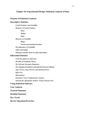
10 - 3To make the comparison more visual, the statistician had prepared a chart of these data (Figure10.1).Figure 10.1 Yards gained or lost by passing and running plays. The mean gain per play, 4yards, is identical for both running and passing plays.What we have in Figure 10.1 are two frequency distributions of yards per play. A frequencydistribution shows the number of times each score (in this case, the number of yards) is obtained.We can tell at a glance that these two distributions are markedly different. A pass play is a study incontrasts; it leads to extremely variable outcomes. Indeed, throwing a pass is somewhat like playingRussian roulette. Large gains, big losses, and incomplete passes (0 gain) are intermingled. A pass
10 - 4doubtless carries with it considerable excitement and apprehension. You never really know what toexpect. On the other hand, a running play is a model of consistency. If it is not exciting, it is at leastdependable. In no case did a run gain more than ten yards, but neither were there any losses. Thesetwo distributions exhibit extremes of variability. In this example, a coach and quarterback wouldprobably pay little attention to measures of central tendency. As we shall see, the fact that the meangain per pass and per run is the same would be of little relevance. What is relevant is the fact that thevariability of running plays is less. It is a more dependable play in a short yardage situation.Seventeen of 20 running plays netted two yards or more. In contrast, only 8 of 20 passing playsgained as much as two yards. Had the situation been different, of course, the decision about whatplay to call might also have been different. If it were the last play in the ball game and 15 yards wereneeded for a touchdown, the pass would be the play of choice. Four times out of 20 a pass gained 15yards or more, whereas a run never came close. Thus, in the strategy of football, variability isfundamental consideration. This is, of course, true of many life situations.Some investors looking for a chance of a big gain will engage in speculative ventures where therisk is large but so, too, is the potential payoff. Others pursue a strategy of investments in blue chipstocks, where the proceeds do not fluctuate like a yo-yo. Many other real-life decisions are based onthe consideration of extremes. A bridge is designed to handle a maximum rather than an averageload; transportation systems and public utilities (such as gas, electric, water) must be prepared tomeet peak rather than average demand in order to avoid shortages and outages.Researchers are also concerned about variability. By and large, from a researcher’s point ofview, variability is undesirable. Like static on an AM radio, it frequently obscures the signal we aretrying to detect. Often the signal of interest in psychological research is a measure of centraltendency, such as the mean, median, or mode.Measures of Central TendencyThe Mean. Two of the most frequently used and most valuable measures of central tendency inpsychological research are the mean and median. Both tell us something about the central values ortypical measure in a distribution of scores. However, because they are defined differently, thesemeasures often take on different values. The mean, commonly known as the arithmetic average,consists of the sum of all scores divided by the number of scores. Symbolically, this is shown asX Xin which X is the mean; the sign directs us to sum the values of the variable X.n(Note: When the mean is abbreviated in text, it is symbolized M). Returning to Table 10.1, we findthat the sum of all yards gained (or lost) by pass plays is 80. Dividing this sum by n (20) yields M
10 - 54. Since the sum of yards gained on the ground is also 80 and n is 20, the mean yards gained percarry is also 4. If we had information only about the mean, our choice between a pass or a run wouldbe up for grabs. But note how much knowledge of variability adds to the decision-making process.When considering the pass play, where the variability is high, the mean is hardly a precise indicatorof the typical gain (or loss). The signal (the mean) is lost in a welter of static (the variability). This isnot the case for the running play. Here, where variability is low, we see that more of the individualmeasures are near the mean. With this distribution, then, the mean is a better indicator of the typicalgain.It should be noted that each score contributes to the determination of the mean. Extreme valuesdraw the mean in their direction. Thus, if we had one running play that gained 88 yards, the sum ofgains would be 160, n would equal 21, and the mean would be 8. In other words, the mean would bedoubled by the addition of one very large gain.The Median. The median does not use the value of each score in its determination. To find themedian, you arrange the values of the variable in order—either ascending or descending—and thencount down (n 1) / 2 scores. This score is the median. If n is an even number, the median ishalfway between the two middle scores. Returning to Table 10.1, we find the median gain on a passplay by counting down to the 10.5th case [(20 1) / 2 10.5)]. This is halfway between the 10th and11th scores. Because both are 0, the median gain is 0. Similarly, the median gain on a running play is3.The median is a particularly useful measure of central tendency when there are extreme scores atone end of a distribution. Such distributions are said to be skewed in the direction of the extremescores. The median, unlike the mean, is unaffected by these scores; thus, it is more likely than themean to be representative of central tendency in a skewed distribution. Variables that haverestrictions at one end of a distribution but not at the other are prime candidates for the median as ameasure of central tendency. A few examples are time scores (0 is the theoretical lower limit andthere is no limit at the upper end), income (no one earns less than 0 but some earn in the millions),and number of children in a family (many have 0 but only one is known to have achieved the recordof 69 by the same mother).The Mode. A rarely used measure of central tendency, the mode simply represents the mostfrequent score in a distribution. Thus, the mode for pass plays is 0, and the mode for running plays is3. The mode does not consider the values of any scores other than the most frequent score. The modeis most useful when summarizing data measured on a nominal scale of measurement. It can also bevaluable to describe a multimodal distribution, one in which the scores tend to occur most frequentlyaround 2 or 3 points in the distribution.
10 - 6Measures of VariabilityWe have already seen that a measure of central tendency by itself provides only a limited amount ofinformation about a distribution. To complete the description, it is necessary to have some idea ofhow the scores are distributed about the central value. If they are widely dispersed, as with the passplays, we say that variability is high. If they are distributed compactly about the central value, as withthe running plays, we refer to the variability as low. But high and low are descriptive words withoutprecise quantitative meaning. Just as we needed a quantitative measure of centrality, so also do werequire a quantitative index of variability.The Range. One simple measure of variability is the range, defined as the difference betweenthe highest and lowest scores in a distribution. Thus, referring to Table 10.1, we see that the range forpass plays is 31 – (–17) 48; for running plays, it is 10 – 0 10. As you can see, the range providesa quick estimate of the variability of the two distributions. However, the range is determined by onlythe two most extreme scores. At times this may convey misleading impressions of total variability,particularly if one or both of these extreme scores are rare or unusual occurrences. For this and otherreasons, the range finds limited use as a measure of variability.The Variance and the Standard Deviation. Two closely related measures of variabilityovercome these disadvantages of the range: variance and standard deviation. Unlike the range,they both make use of all the scores in their computation. Indeed, both are based on the squareddeviations of the scores in the distribution from the mean of the distribution.Table 10.2 illustrates the number of aggressive behaviors during a one-week observation periodfor two different groups of children. The table includes measures of central tendency and measures ofvariability. Note that the symbols and formulas for variance and standard deviation are those that usesample data to provide estimates of variability in the population.
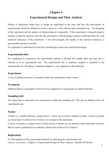
10 - 7Notice that although the measures of central tendency are identical for both groups of scores,the measures of variability are not and reflect the greater spread of scores in Group 2. This isapparent in all three measures of variability (range, variance, standard deviation). Also notice that thevariance is based on the squared deviations of scores from the mean and that the standard deviation issimply the square root of the variance. For most sets of scores that are measured on an interval orratio scale of measurement, the standard deviation is the preferred measure of variability.Conceptually, you should think of standard deviation as “on average, how far scores are from themean.”Now, if the variable is distributed in a bell-shaped fashion known as the normal curve, therelationships can be stated with far more precision. Approximately 68% of the scores lie between themean and 1 standard deviation, approximately 95% of the scores lie between 2 standarddeviations, and approximately 98% of the scores lie between 3 standard deviations. These featuresof normally distributed variables are summarized in Figure 10.2.
10 - 8Figure 10.2 Areas between the mean and selected numbers of standard deviations above andbelow the mean for a normally distributed variable.Note that these areas under the normal curve can be translated into probability statements.Probability and proportion are simply percentage divided by 100. The proportion of area foundbetween any two points in Figure 10.2 represents the probability that a score, drawn at random fromthat population, will assume one of the values found between these two points. Thus, the probabilityof selecting a score that falls between 1 and 2 standard deviations above the mean is 0.1359.Similarly, the probability of selecting a score 2 or more standard deviations below the mean is 0.0228(0.0215 .0013).Many of the variables with which psychologists concern themselves are normally distributed,such as standardized test scores. What is perhaps of greater significance for the researcher is the factthat distributions of sample statistics tend toward normality as sample size increases. This is trueeven if the population distribution is not normal. Thus, if you were to select a large number ofsamples of fixed sample size, say n 30, from a nonnormal distribution, you would find that separateplots of their means, medians, standard deviations, and variances would be approximately normal.The Importance of VariabilityWhy is variability such an important concept? In research, it represents the noisy background out ofwhich we are trying to detect a coherent signal. Look again at Figure 10.1. Is it not clear that themean is a more coherent representation of the typical results of a running play than is the mean of a
10 - 9pass play? When variability is large, it is simply more difficult to regard a measure of centraltendency as a dependable guide to representative performance.This also applies to detecting the effects of an experimental treatment. This task is very muchlike distinguishing two or more radio signals in the presence of static. In this analogy, the effects ofthe experimental variable (treatment) represent the radio signals, and the variability is the static(noise). If the radio signal is strong, relative to the static, it is easily detected; but if the radio signal isweak, relative to the static, the signal may be lost in a barrage of noise.In short, two factors are commonly involved in assessing the effects of an experimentalvariable: a measure of centrality, such as the mean, median, or proportion; and a measure ofvariability, such as the standard deviation. Broadly speaking, the investigator exercises little controlover the measure of centrality. If the effect of the treatment is large, the differences in measures ofcentral tendency will generally be large. In contrast, control over variability is possible. Indeed, muchof this text focuses, directly or indirectly, on procedures for reducing variability—for example,selecting a reliable dependent variable, providing uniform instructions and standardized experimentalprocedures, and controlling obtrusive and extraneous experimental stimuli. We wish to limit theextent of this unsystematic variability for much the same reasons that a radio operator wishes to limitstatic or noise—to permit better detection of a treatment effect in the one case and a radio signal inthe other. The lower the unsystematic variability (random error), the more sensitive is our statisticaltest to treatment effects.Tables and GraphsRaw scores, measures of central tendency, and measures of variability are often presented in tables orgraphs. Tables and graphs provide a user-friendly way of summarizing information and revealingpatterns in the data. Let’s take a hypothetical set of data and play with it.One group of 30 children was observed on the playground after watching a TV program withoutviolence, and another group of 30 children was observed on the playground after watching a TVprogram with violence. In both cases, observers counted the number of aggressive behaviors. Thedata were as follows:Program with no violence: 5, 2, 0, 4, 0, 1, 2, 1, 3, 6, 5, 1, 4, 2, 3, 2, 2, 2, 5, 3, 4, 2, 2, 3, 4, 3, 7, 3, 6,3, 3Program with violence: 5, 3, 1, 4, 2, 0, 5, 3, 4, 2, 6, 1, 4, 1, 5, 3, 7, 2, 4, 2, 3, 5, 4, 6, 3, 4, 4, 5, 6, 5Take a look at the raw scores. Do you see any difference in number of aggressive behaviors betweenthe groups? If you are like us, you find it difficult to tell.
10 - 10One of the first ways we might aid interpretation is to place the raw scores in a table called afrequency distribution and then translate that same information into a graph called a frequencyhistogram (see Figure 10.3).Figure 10.3 Number of aggressive behaviors illustrated in both frequency distributions andfrequency histograms.Both the frequency distribution and the frequency histogram in Figure 10.3 make it easy todetect the range of scores, the most frequent score (mode), and the shape of the distribution. A quick
10 - 11glance at the graphs now suggests that the children tended to exhibit fewer aggressive behaviors afterthe TV program with no violence. We can further summarize the data by calculating the mean andstandard deviation for each group and presenting these values in both a table and a figure (see Table10.3 and Figure 10.4).Figure 10.4 Graphical depiction of the mean and standard deviation for the No Violence andViolence groups.In Figure 10.4, the mean is depicted by a square, and the bars represent 1 standard deviationabove and below the mean. Thus, although the means differ by 0.6 units, one can see from thestandard deviation bars that there is quite a bit of overlap between the two sets of scores. Inferentialstatistics will be needed to determine whether the difference between the means is statisticallysignificant.
10 - 12In the preceding description of data, we selected a few ways that the data could be summarizedin both tables and figures. However, these methods are certainly not exhaustive. We can displaythese data and other data in a variety of other ways, in both tabular and graphical form, and weencourage students to experiment with these techniques. Remember that the data are your windowinto participant behavior and thought. You can only obtain a clear view by careful examination of thescores.Before we turn to inferential statistics, let’s think about the added clarity that descriptivestatistics can provide when observed behavior is described. To do this, we return to the report of astudy that was first described in Chapter 6 and is considered again here in the box “ThinkingCritically About Everyday Information.”Thinking Critically About Everyday Information: School Backpacks and Posture RevisitedA news report by MSNBC describes a study in which children were observed carrying schoolbackpacks. The article states:Thirteen children ages 8 and 9 walked about 1,310 feet without a backpack, andwearing packs weighing 9 and 13 pounds, while researchers filmed them with a highspeed camera. . . . The kids did not change their strides, the images showed. Instead,the youngsters bent forward more as they tried to counter the loads on their backs,and the heavier loads made them bend more, the study found. As they grew moretired, their heads went down, Orloff said.In Chapter 6, we focused our critical thinking questions on the method of observation. Now,let’s think about the description of the observations: The article states that when children carried the backpacks, they “did not change their strides” but“bent forward more.” Although this description is typical of a brief news report, what specificmeasure of central tendency could be reported for each dependent variable to clarify thedescription?What measure of variability would clarify the description?How would you create a graph that would nicely summarize the pattern of results reported in thearticle?Why is it that most reports of research in the everyday media do not report measures of centraltendency and variability, with related tables or graphs?Retrieved June 11, 2003. online at http://www.msnbc.com/news/922623.asp?0si -
10 - 13Inferential StatisticsFrom Descriptions to InferencesWe have examined several descriptive statistics that we use to make sense out of a mass of raw data.We have briefly reviewed the calculation and interpretation of statistics that are used to describe boththe central tendency of a distribution of scores or quantities (mean, median, and mode) and thedispersion of scores around the central tendency (range, standard deviation, and variance). Our goalin descriptive statistics is to describe, with both accuracy and economy of statement, aspects ofsamples selected from the population.It should be clear that our primary focus is not on the sample statistics themselves. Their valuelies primarily in the light that they may shed on characteristics of the population. Thus, we are notinterested, as such, in the fact that the mean of the control group was higher or lower than the meanof an experimental group, nor that a sample of 100 voters revealed a higher proportion favoringCandidate A. Rather, our focus shifts from near to far vision; it shifts from the sample to thepopulation. We wish to know if we may justifiably conclude that the experimental variable has hadan effect; or we wish to predict that Candidate A is likely to win the election. Our descriptivestatistics provide the factual basis for the inductive leap from samples to populations.In the remainder of this chapter, we will take a conceptual tour of statistical decision making.The purpose is not to dwell on computational techniques but rather to explore the rationaleunderlying inferential statistics.The Role of Probability TheoryRecall the distinction between deductive and inductive reasoning. With deductive reasoning, the truthof the conclusion is implicit in the assumptions. Either we draw a valid conclusion from thepremises, or we do not. There is no in-between ground. This is not the case with inductive orscientific proof. Conclusions do not follow logically from a set of premises. Rather, they representextensions of or generalizations based on empirical observations. Hence, in contrast to logical proof,scientific or inductive conclusions are not considered valid or invalid in any ultimate sense. Ratherthan being either right or wrong, we regard scientific propositions as having a given probability ofbeing valid. If observation after observation confirms a proposition, we assign a high probability(approaching 1.00) to the validity of the proposition. If we have deep and abiding reservations aboutits validity, we may assign a probability that approaches 0. Note, however, we never establishscientific truth, nor do we disprove its validity, with absolute certainty.Most commonly, probabilities are expressed either as a proportion or as a percentage. As theprobability of an event approaches 1.00, or 100%, we say that the event is likely to occur. As it
10 - 14approaches 0.00, or 0%, we deem the event unlikely to occur. One way of expressing probability isin terms of the number of events favoring a given outcome relative to the total number of eventspossible. Thus,PA number of events favoring Anumber of events favoring A number of events not favoring ATo illustrate, if a population of 100,000 individuals contains 10 individuals with the disorderphenylketonuria (PKU), what is the probability that a person, selected at random, will have PKU?PPKU 10 0.0001 or 0.01%10 99,990Thus, the probability is extremely low: 1 in 10,000.This definition is perfectly satisfactory for dealing with discrete events (those that are counted).However, how do we define probability when the variables are continuous—for example, weight, IQscore, or reaction time? Here, probabilities can be expressed as a proportion of one area under acurve relative to the total area under a curve. Recall the normal distribution. The total area under thecurve is 1.00. Between the mean and 1 standard deviation above the mean, the proportion of the totalarea is 0.3413. If we selected a sample score from a normally distributed population, what is theprobability that it would be between the mean and 1 standard deviation above the mean? Becauseabout 34% of the total area is included between these points, p 0.34. Similarly, p 0.34 that asingle randomly selected score would be between the mean and 1 standard deviation below the mean.Figure 10.2 shows areas under the standard normal curve and permits the expression of any value ofa normally distributed variable in terms of probability.Probability looms large on the scene of inferential statistics because it is the basis for acceptingsome hypotheses and rejecting others.The Null and Alternative HypothesesBefore beginning an experiment, the researcher sets up two mutually exclusive hypotheses. One is astatistical hypothesis that the experimenter expects to reject. It is referred to as the null hypothesisand is usually represented symbolically as Ho. The null hypothesis states some expectation regardingthe value of one or more population parameters. Most commonly, it is a hypothesis of no difference(no effect). Let us look at a few examples:
10 - 15 If we were testing the honesty of a coin, the null hypothesis (Ho) would read: The coinis unbiased. Stated more precisely, the probability of a head is equal to the probabilityof a tail: Ph Pt ½ 0.5. If we were evaluating the effect of a drug on reaction time, the null hypothesis mightread: The drug has no effect on reaction time.The important point to remember about the null hypothesis is that it always states someexpectation regarding a population parameter—such as the population mean, median, proportion,standard deviation, or variance. It is never stated in terms of expectations of a sample. For example,we would never state that the sample mean (or median or proportion) of one group is equal to thesample mean of another. It is a fact of sampling behavior that sample statistics are rarely identical,even if selected from the same population. Thus, ten tosses of a single coin will not always yield fiveheads and five tails. The discipline of statistics sets down the rules for making an inductive leap fromsample statistics to population parameters.The alternative hypothesis (H1) denies the null hypothesis. If the null hypothesis states thatthere is no difference in the population means from which two samples were drawn, the alternativehypothesis asserts that there is a difference. The alternative hypothesis usually states theinvestigator’s expectations. Indeed, there really would be little sense embarking upon costly andtime-consuming research unless we had some reason for expecting that the experimental variable willhave an effect. Let’s look at a few examples of alternative hypotheses: In the study aimed at testing the honesty of a coin, the alternative hypothesis wouldread: H1: Ph Pt 1/2; the probability of a head is not equal to the probability of a tail,which is not equal to one-half. In the effect of a drug on reaction time, the alternative hypothesis might read: Theadministration of a given dosage level of a drug affects reaction time.The Sampling Distribution and Statistical Decision MakingNow that we have stated our null and alternative hypotheses, where do we go from here? Recall thatthese hypotheses are mutually exclusive. They are also exhaustive. By exhaustive we mean that noother possibility exists. These two possible outcomes in our statistical decision exhaust all possibleoutcomes. If the null hypothesis is true, then the alternative hypothesis must be false. Conversely, ifthe null hypothesis is false, then the alternative hypothesis must be true.
10 - 16Considering these realities, our strategy would appear to be quite straightforward—simplydetermine whether the null hypothesis is true or false. Unfortunately, there is one further wrinkle.The null hypothesis can never be proved to be true. How would you go about proving that a drug hasno effect, or that males and females are equally intelligent, or that a coin is honest? If you flipped it1,000,000 times and obtained exactly 500,000 heads, wouldn’t that be proof positive? No. It wouldmerely indicate that, if a bias does exist, it must be exceptionally small. But we cannot rule out thepossibility that a small bias does exist. Perhaps the next million, 5 million, or 10 billion tosses willreveal this bias. So we have a dilemma. If we have no way of proving one of two mutually exclusiveand exhaustive hypotheses, how can we establish which of these alternatives has
In previous chapters, we have discussed the basic principles of good experimental design. Before examining specific experimental designs and the way that their data are analyzed, we thought that it would be a good idea to review some basic principles of statistics. We assume that most of