WIXLIB

Probability Properties PX(xi): the probability of the random variable X taking onthe value xi The probability of an event to happen is a non-negativenumber, with the following properties:– The probability of the event that includes all possible outcomes ofthe experiment is 1.– The probability of two events that do not have any commonoutcome is the sum of the probabilities of the two eventsseparately. Example– Roll a die:PX(x k) 1/6for k 1, 2, , 629

CDF and PDF The (cumulative) distribution function (cdf) of a random variable Xis defined as the probability of X taking a value less than theargumentt x:FX ( x) P( X x) PropertiesFX ( ) 0, FX ( ) 1FX ( x1 ) FX ( x2 ) if x1 x2 The probability density function (pdf) is defined as the derivative ofthe distribution function:f X ( x) dF X ( x )dxxFX ( x ) f X ( y ) dy bP ( a X b ) FX (b ) FX ( a ) f X ( y ) dyaf X ( x) dF X ( x )dx 0 since F X ( x ) is non - decreasing30

Mean and Variance If x is sufficiently small,P ( x X x x ) x xf X ( y) f X ( y ) dy f X ( x ) xxAreaf X ( x) xyx Mean (or expected value DC level):E[ X ] X x f X ( x ) dxE[ ]: expectationoperatorVariance ( power for zero-mean signals): X2 E[( X X ) 2 ] ( x X ) 2 f X ( x)dx E[ X 2 ] X2 31

Normal (Gaussian) Distributionf X ( x) m0f X ( x) FX ( x ) 12 12 e ( x m )22 2x e ( y m )22 2f x fordyxE[ X ] m X2 2 : rm s v a lu e32

Uniform DistributionfX(x) 1 f X ( x) b a 0 0 x a FX ( x ) b a 1a x belsewherex aa x ba b2(b a ) 2 12E[ X ] X2x b33

Joint Distribution Joint distribution function for two random variables X and YFXY ( x , y ) P ( X x , Y y ) Joint probability density functionf XY ( x, y ) Properties 2 FXY ( x , y ) x y 1) FXY ( , ) f XY (u , v)dudvd d 1 2)f X ( x) f XY ( x, y ) dyy 3)fY ( x ) f XY ( x, y ) dxx 4)X , Y are independent f XY ( x, y ) f X ( x) fY ( y )5)X , Y are uncorrelated E[ XY ] E[ X ]E[Y ]34

Independent vs. Uncorrelated Independent implies Uncorrelated (see problem sheet) Uncorrelated does not imply Independence For normal RVs (jointly Gaussian), Uncorrelated impliesIndependent (this is the only exceptional case!) An example of uncorrelated but dependent RV’sLet be uniformlyy distributed in [0,2 ]f ( x) 21 for 0 x 2 YDefine RV’s X and Y asX cos Y sin Clearly,y, X and Y are not independent.pBut X and Y are uncorrelated:E[ XY ] 12 2 0Locus ofX and YXcos sin d 0!35

Joint Distribution of n RVs Joint cdfFX1 X 2 . X n ( x1 , x2 ,.xn ) P( X 1 x1 , X 2 x2 ,. X n xn ) Joint pdff X 1 X 2 . X n ( x1 , x2 ,.xn ) n FX1X 2 . X n ( x1 , x2 ,. xn ) x1 x2 . xn IndependentFX 1 X 2 . X n ( x1 , x2 ,.xn ) FX 1 ( x1 ) FX 2 ( x2 ).FX n ( xn )f X 1 X 2 . X n ( x1 , x2 ,.xn ) f X 1 ( x1 ) f X 2 ( x2 ).) f X n ( xn ) i.i.d. (independent, identically distributed)– The random variables are independent and have the samedistribution.– Example: outcomes from repeatedly flipping a coin.36

Central Limit Theorem For i.i.d. random variables,z x1 x2 · · · xntends to Gaussian as ngoes to infinity. Extremely useful incommunications. That’s why noise is usuallyGaussian. We often say“GaussianGaussian noise”noise or“Gaussian channel” incommunications.x1x1 x2 x3x1 x2x1 x2 x3 x4Illustration of convergence to Gaussiandistribution37

What is a Random Process? A random process is a time-varying function that assignsthe outcome of a random experiment to each time instant:X(t). For a fixed (sample path): a random process is a timevarying function, e.g., a signal. For fixed t: a random pprocess is a random variable. If one scans all possible outcomes of the underlyingrandom experiment, we shall get an ensemble of signals. Noise can often be modelled as a Gaussian randomprocess.38

An Ensemble of Signals39

Statistics of a Random Process For fixed t: the random process becomes a randomvariable, with mean X (t ) E[ X (t )] x f X ( x; t )dx – In generalgeneral, the mean is a function of t.t Autocorrelation functionRX (t1 , t2 ) E[ X (t1 ) X (t2 )] xy f X ( x, y; t1 , t2 )dxdy– In general, the autocorrelation function is a two-variable function.– It measures the correlation between two samples.40

Stationary Random Processes A random process is (wide-sense) stationary if– Its mean does not dependpon t X (t ) X– Its autocorrelation function only depends on time differenceRX (t, t ) RX ( ) In communications,, noise and messageg signalsgcan oftenbe modelled as stationary random processes.41

Example Show that sinusoidal wave with random phaseX (t ) A cos(( c t )with phase Θ uniformly distributed on [0,2π] is stationary.– Mean is a constant:12 f ( ) , [0[0, 2 ]1 X (t ) E[ X (t )] A cos( ct ) d 02 02 – Autocorrelation function only depends on the time difference:RX (t , t ) E[ X (t ) X (t )] E[ A2 cos( c t ) cos( c t c )]A2A2 E[cos(2 c t c 2 )] E[cos( c )]22A2 2 1A2 cos(2 c t c 2 )d cos( c ) 022 2A2RX ( ) cos( c )242

Power Spectral Density Power spectral density (PSD) is a function that measuresthe distribution of power of a random process withfrequency. PSD is only defined for stationary processes. Wiener-KhinchineWiener Khinchine relation: The PSD is equal to theFourier transform of its autocorrelation function: S X ( f ) R X ( )e j 2 f d – A similar relation exists for deterministic signals Then the average power can be found as 2P E[ X (t )] R X (0) S X ( f )df TheTh frequencyfcontent off a process dependsdd on howhrapidly the amplitude changes as a function of time.– This can be measured by the autocorrelation functionfunction.43

Passing Through a Linear System LLett Y(t) obtainedbt i d bby passingi randomdprocess X(t) ththroughha linear system of transfer function H(f). Then the PSD ofY(t)2(2.1)SY ( f ) H ( f ) S X ( f )– Proof: see Notes 33.4.2.42– Cf. the similar relation for deterministic signals If X(t)( ) is a Gaussian pprocess,, then Y(t)( ) is also a Gaussianprocess.– Gaussian processes are very important in communications.44

EE2--4: Communication SystemsEE2Lecture 3: NoiseDr. Cong LingDepartment of Electrical and Electronic Engineering45

Outline What is noise?White noise and Gaussian noiseLowpass noiseBandpass noise– In-phase/quadrature representation– Phasor representationp References– Notes of Communication Systems, Chap. 2.– Haykin & Moher, Communication Systems, 5th ed., Chap. 5– Lathi, Modern Digital and Analog Communication Systems, 3rd ed.,Chap. 1146

Noise Noise is the unwanted and beyond our control waves thatgdisturb the transmission of signals. Where does noise come from?– External sources: e.g., atmospheric, galactic noise, interference;– Internal sources: generated by communication devices themselves. This type of noise represents a basic limitation on the performance ofelectronic communication systemssystems. Shot noise: the electrons are discrete and are not moving in acontinuous steady flow, so the current is randomly fluctuating. ThermalThl noise:icauseddbby ththe rapidid andd randomdmotionti off electronsl twithin a conductor due to thermal agitation. Both are often stationaryy and have a zero-mean Gaussiandistribution (following from the central limit theorem).47

White Noise The additive noise channel– n(t)( ) models all typesyp of noise– zero mean White noise– Its power spectrum density (PSD) is constant over all frequencies,i.e.,N f SN ( f ) 0 ,2– Factor 1/2 is included to indicate that half the power is associatedwith positive frequencies and half with negative.– The term white is analogous to white light which contains equalamounts of all frequencies (within the visible band of EM wave).– ItIt’ss only defined for stationary noisenoise. An infinite bandwidth is a purely theoretic assumption.48

White vs. Gaussian Noise White noiseSN(f)PSDRn( )N– Autocorrelation function of n(t ) : Rn ( ) 0 ( )2– SamplesSl att diffdifferentt timetiiinstantst t are uncorrelated.l t d Gaussian noise: the distribution at any time instant isGaussianGaussian– Gaussian noise can be colored White noise Gaussian noisePDF– White noise can be non-Gaussian Nonetheless, in communications, it is typically additivewhite Gaussian noise (AWGN)(AWGN).49

Ideal LowLow--Pass White Noise Suppose white noise is applied to an ideal low-pass filterof bandwidth B such that N0 , f BSN ( f ) 2 0,otherwisePower PN N0B ByB Wiener-KhinchineWiKhi hi relation,l iautocorrelationl i ffunctioniRn( ) E[n(t)n(t )] N0B sinc(2B )(3.1)where sinc(x) sin( x)/ x.x Samples at Nyquist frequency 2B are uncorrelatedRn( ) 0,0 k/(2B),k/(2B) k 1,1 2,2 50

Bandpass Noise Any communication system that uses carrier modulation will typicallyhave a bandpass filter of bandwidth B at the front-end of the receiver.n(t) Anyy noise that enters the receiver will therefore be bandpasspin nature:its spectral magnitude is non-zero only for some band concentratedaround the carrier frequency fc (sometimes called narrowband noise).51

Example If white noise with PSD of N0/2 is passed through an idealbandpasspfilter,, then the PSD of the noise that enters thereceiver is given by N0 , f fC BSN ( f ) 2 0,otherwisePower PN 2N0B Autocorrelation functionRn( ) 2N0Bsinc(2B )cos(2 fc )– which follows from (3.1) byapplyingl i ththe ffrequency-shifthiftproperty of the Fourier transformg ( t ) G ( )g ( t ) 2 cos 0 t [ G ( 0 ) G ( 0 )] Samples taken at frequency 2B are still uncorrelated.uncorrelatedRn( ) 0, k/(2B), k 1, 2, 52

Decomposition of Bandpass Noise Consider bandpass noise within f fC B with any PSD((i.e.,, not necessarilyy white as in the previouspexample)p ) Consider a frequency slice f at frequencies fk and fk. For f small:n k ( t ) a k cos( 2 f k t k )– θk: a random pphase assumed independentpand uniformlyydistributed in the range [0, 2 )– ak: a random amplitude. f-ffkfk53

Representation of Bandpass Noise The complete bandpass noise waveform n(t) can beconstructed by summing up such sinusoids over the entireband ii.e.,band,en(t ) nk (t ) ak cos(2 f k t k )kf k f c k f(3.2)k Now, let fk (fk fc) fc, and using cos(A B) cosAcosB sinAsinB we obtain the canonical form of bandpassnoisein(t ) nc (t ) cos(2 f ct ) ns (t ) sin( 2 f ct )wherenc (t ) ak cos(2 ( f k f c )t k )k(3.3)ns (t ) ak sin( 2 ( f k f c )t k )k– nc(t) and ns(t) are baseband signals,signals termed the in-phasein phase andquadrature component, respectively.54

Extraction and Generation nc(t) and ns(t) are fully representative of bandpass noise.– (a)( ) Given bandpasspnoise,, one mayy extract its in-phasepandquadrature components (using LPF of bandwith B). This isextremely useful in analysis of noise in communication receivers.– (b) Given the two components,components one may generate bandpass noisenoise.This is useful in computer simulation.nc(t)nc(t)ns(t)ns(t)55

Properties of Baseband Noise If the noise n(t) has zero mean, then nc(t) and ns(t) havezero mean. If the noise n(t) is Gaussian, then nc(t) and ns(t) areGaussian. If the noise n(t) is stationary, then nc(t) and ns(t) arestationary. If the noise n(t) is Gaussian and its power spectral densityS( f ) is symmetric with respect to the central frequency fc,th nc(t)then( ) andd ns(t)( ) are statisticalt ti ti l independent.i dd t The components nc(t) and ns(t) have the same variance ( power) as n(t).)56

Power Spectral Density Further, each baseband noise waveform will have thesame PSD: S N ( f f c ) S N ( f f c ), f BSc ( f ) S s ( f ) otherwise 0,(3.4) This is analogous tog (t ) G ( )g (t )2 cos 0t [G ( 0 ) G ( 0 )]– A rigorousgpproof can be found in A. Papoulis,p, Probability,y, RandomVariables, and Stochastic Processes, McGraw-Hill.– The PSD can also be seen from the expressions (3.2) and (3.3)where each of nc(t) and ns(t) consists of a sum of closely spacedbase-band sinusoids.57

Noise Power For ideally filtered narrowband noise, the PSD of nc(t)Sc(f) Ss(f)and ns((t)) is therefore ggiven byy N 0 , f BSc ( f ) S s ( f ) 0, otherwise(3.5) Corollary: The average power in each of the basebandwaveformsfnc(t)( ) andd ns(t)( ) isi identicalid ti l tot theth average powerin the bandpass noise waveform n(t). For ideally filtered narrowband noisenoise, the variance of nc(t)and ns(t) is 2N0B each.PNc PNs 2N0B58

Phasor Representation We may write bandpass noise in the alternative form:n(t ) nc (t ) cos(2 f c t ) ns (t ) sin(2 f c t ) r (t ) cos[2 f c t (t )]––r (t ) nc (t ) 2 ns (t ) 2 ns ( t ) nc (t ) (t ) tan 1 : the envelop of the noise: the pphase of the noiseθ( ) 2 fct (t)θ(t)()59

Distribution of Envelop and Phase It can be shown that if nc(t) and ns(t) are Gaussiangr(t)( ) has a Rayleighy gdistributed,, then the magnitudedistribution, and the phase (t) is uniformly distributed. What if a sinusoid Acos(2 fct) is mixed with noise? Then the magnitudegwill have a Rice distribution. The pproof is deferred to Lecture 11,, where suchdistributions arise in demodulation of digital signals.60

Summary White noise: PSD is constant over an infinite bandwidth. Gaussian noise: PDF is GaussianGaussian. Bandpass noise– In-phaseIn phase and quadrature compoments nc(t) and ns(t) are low-passlow passrandom processes.– nc(t) and ns(t) have the same PSD.– nc(t) and ns(t) have the same variance as the band-pass noise n(t).– Such properties will be pivotal to the performance analysis ofbandpass communication systems. The in-phase/quadrature representation and phasorrepresentationpare not onlyy basic to the characterization ofbandpass noise itself, but also to the analysis of bandpasscommunication systems.61

EE2--4: Communication SystemsEE2Lecture 4: Noise Performance of DSBDr. Cong LingDepartment of Electrical and Electronic Engineering62

Outline SNR of baseband analog transmission Revision of AM SNR of DSB-SC References– Notes of Communication SystemsSystems, ChapChap. 33.1-3.3.2.1-3 3 2– Haykin & Moher, Communication Systems, 5th ed., Chap. 6– Lathi, Modern Digital and Analog Communication Systems, 3rd ed.,Chap. 1263

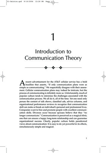
Noise in Analog Communication Systems How do various analog modulation schemes perform inthe presence of noise? Which scheme performs best? How can we measure its performance?Model of an analog communication systemNoise PSD: BT is the bandwidth,N0/2 is the double-sided noise PSD64

SNR We must find a way to quantify ( to measure) theperformance of a modulation scheme.p We use the signal-to-noise ratio (SNR) at the output of thereceiver:average power of message signal at the receiver output PSSNRo average power of noise at the receiver outputPN– Normally expressed in decibels (dB)– SNR (dB) 10 log10(SNR)– This is to manage the wide range of powerlevels in communication systems– In honour of Alexander Bell– Example:pdBIf x is power,X (dB) 10 log10(x)If x is amplitude,X ((dB)) 20 logg10((x)) ratio of 2 3 dB; 4 6 dB; 10 10dB65

Transmitted Power PT: The transmitted power Limited by: equipment capabilitycapability, battery lifelife, costcost,government restrictions, interference with other channels,green communications etc The higher it is, the more the received power (PS), thehigher the SNR For a fair comparison between different modulationschemes:– PT should be the same for all We use the baseband signal to noise ratio SNRbaseband tocalibrate the SNR values we obtain66

A Baseband Communication System It does not usemodulation It is suitable fortransmission over wires The power it transmitsis identical to themessage power: PT P No attenuation: PS PT P The results can beextended to bandband-passpasssystems67

Output SNR Average signal ( message) powerP the area under the triangular curveAssume: Additive, white noise with power spectraldensity PSD N0/2AAveragenoiseipower att ththe receiveriPN area under the straight line 2W N0/2 WN0SNR at the receiver output:SNRbasebandPT N 0W– Note: Assume no propagation loss Improve the SNR by:– increasing the transmitted power (PT ),– restricting the message bandwidth (W ),– making the channel/receiver less noisy (N0 ). )68

Revision: AM General form of an AM signal:s(t ) AM [ A m(t )] cos(2 f ct )– AA: theth amplitudelit d off theth carrieri– fc: the carrier frequency– m(t): the message signal Modulation index: mpA– mp: the peak amplitude of m(t), i.e., mp max m(t) 69

Signal Recoveryn(t)Receiver model1) 1 A m p : use an envelopelddetector.t tThis is the case in almost all commercial AM radioreceiversreceivers.Simple circuit to make radio receivers cheap.2) Otherwise: use synchronous detection productdetection coherent detectionTh termsThetdetectiond t ti andd demodulationdd l ti are usedd iinterchangeably.t hbl70

Synchronous Detection for AM Multiply the waveform at the receiver with a local carrier ofthe same frequency (and phase) as the carrier used at thettransmitter:itt2 cos(2 f c t ) s (t ) AM [ A m(t )]2 cos 2 (2 f c t ) [ A m(t )][1 cos(4 f c t )] A m(t ) Use a LPF to recover A m(t) and finally m(t) Remark: At the receiver you need a signal perfectlysynchronized with the transmitted carrier71

DSB--SCDSB Double-sideband suppressed carrier (DSB-SC)s (t ) DSB SC Am(t ) cos(2 f c t ) Signal recovery: with synchronous detection only The received noisy signal isx (t ) s (t ) n (t ) s(t ) nc (t ) cos(2 f c t ) ns (t ) sin(2 f c t ) Am(t ) cos(2 f c t ) nc (t ) cos(2 f c t ) ns (t ) sin(2 f ct ) [ AmA (t ) nc (t )] cos((2 f c t ) ns (t ) sin(i (2 f c t )y(t)272

Synchronous Detection for DSBDSB-SC Multiply with 2cos(2fct):y (t ) 2 cos(2 f c t ) x(t ) Am(t )2 cos 2 (2 f c t ) nc (t )2 cos 2 (2 f c t ) ns (t ) sin(4 f c t ) Am(t )[1 cos(4 f c t )]

Communication Systems mostly deals with the physical layer but 24 Communication Systems mostly deals with the physica