Transcription
An Introduction to Genetic AlgorithmsJenna CarrMay 16, 2014AbstractGenetic algorithms are a type of optimization algorithm, meaning they are used tofind the maximum or minimum of a function. In this paper we introduce, illustrate,and discuss genetic algorithms for beginning users. We show what components makeup genetic algorithms and how to write them. Using MATLAB, we program severalexamples, including a genetic algorithm that solves the classic Traveling SalesmanProblem. We also discuss the history of genetic algorithms, current applications, andfuture developments.Genetic algorithms are a type of optimization algorithm, meaning they are used to findthe optimal solution(s) to a given computational problem that maximizes or minimizes aparticular function. Genetic algorithms represent one branch of the field of study calledevolutionary computation [4], in that they imitate the biological processes of reproductionand natural selection to solve for the ‘fittest’ solutions [1]. Like in evolution, many of agenetic algorithm’s processes are random, however this optimization technique allows one toset the level of randomization and the level of control [1]. These algorithms are far morepowerful and efficient than random search and exhaustive search algorithms [4], yet requireno extra information about the given problem. This feature allows them to find solutionsto problems that other optimization methods cannot handle due to a lack of continuity,derivatives, linearity, or other features.1
Section 1 explains what makes up a genetic algorithm and how they operate. Section 2walks through three simple examples. Section 3 gives the history of how genetic algorithmsdeveloped. Section 4 presents two classic optimization problems that were almost impossibleto solve before the advent of genetic algorithms. Section 5 discusses how these algorithmsare used today.1Components, Structure, & TerminologySince genetic algorithms are designed to simulate a biological process, much of the relevantterminology is borrowed from biology. However, the entities that this terminology refersto in genetic algorithms are much simpler than their biological counterparts [8]. The basiccomponents common to almost all genetic algorithms are: a fitness function for optimization a population of chromosomes selection of which chromosomes will reproduce crossover to produce next generation of chromosomes random mutation of chromosomes in new generationThe fitness function is the function that the algorithm is trying to optimize [8]. The word“fitness” is taken from evolutionary theory. It is used here because the fitness function testsand quantifies how ‘fit’ each potential solution is. The fitness function is one of the mostpivotal parts of the algorithm, so it is discussed in more detail at the end of this section. Theterm chromosome refers to a numerical value or values that represent a candidate solutionto the problem that the genetic algorithm is trying to solve [8]. Each candidate solution isencoded as an array of parameter values, a process that is also found in other optimizationalgorithms [2]. If a problem has Npar dimensions, then typically each chromosome is encoded2
as an Npar -element arraychromosome [p1 , p2 , ., pNpar ]where each pi is a particular value of the ith parameter [2]. It is up to the creator of thegenetic algorithm to devise how to translate the sample space of candidate solutions intochromosomes. One approach is to convert each parameter value into a bit string (sequenceof 1’s and 0’s), then concatenate the parameters end-to-end like genes in a DNA strandto create the chromosomes [8]. Historically, chromosomes were typically encoded this way,and it remains a suitable method for discrete solution spaces. Modern computers allowchromosomes to include permutations, real numbers, and many other objects; but for nowwe will focus on binary chromosomes.A genetic algorithm begins with a randomly chosen assortment of chromosomes, whichserves as the first generation (initial population). Then each chromosome in the populationis evaluated by the fitness function to test how well it solves the problem at hand.Now the selection operator chooses some of the chromosomes for reproduction based ona probability distribution defined by the user. The fitter a chromosome is, the more likely itis to be selected. For example, if f is a non-negative fitness function, then the probabilitythat chromosome C53 is chosen to reproduce might bef (C53 ).P (C53 ) PNpopi 1 f (Ci )Note that the selection operator chooses chromosomes with replacement, so the same chromosome can be chosen more than once. The crossover operator resembles the biologicalcrossing over and recombination of chromosomes in cell meiosis. This operator swaps asubsequence of two of the chosen chromosomes to create two offspring. For example, if theparent chromosomes[11010111001000] and [01011101010010]3
are crossed over after the fourth bit, then[01010111001000] and [11011101010010]will be their offspring. The mutation operator randomly flips individual bits in the newchromosomes (turning a 0 into a 1 and vice versa). Typically mutation happens with a verylow probability, such as 0.001. Some algorithms implement the mutation operator beforethe selection and crossover operators; this is a matter of preference. At first glance, themutation operator may seem unnecessary. In fact, it plays an important role, even if itis secondary to those of selection and crossover [1]. Selection and crossover maintain thegenetic information of fitter chromosomes, but these chromosomes are only fitter relativeto the current generation. This can cause the algorithm to converge too quickly and lose“potentially useful genetic material (1’s or 0’s at particular locations)” [1]. In other words,the algorithm can get stuck at a local optimum before finding the global optimum [3].The mutation operator helps protect against this problem by maintaining diversity in thepopulation, but it can also make the algorithm converge more slowly.Typically the selection, crossover, and mutation process continues until the number ofoffspring is the same as the initial population, so that the second generation is composedentirely of new offspring and the first generation is completely replaced. We will see thismethod in Examples 2.1 and 2.2. However, some algorithms let highly-fit members of thefirst generation survive into the second generation. We will see this method in Example 2.3and Section 4.Now the second generation is tested by the fitness function, and the cycle repeats. It isa common practice to record the chromosome with the highest fitness (along with its fitnessvalue) from each generation, or the “best-so-far” chromosome [5].Genetic algorithms are iterated until the fitness value of the “best-so-far” chromosomestabilizes and does not change for many generations. This means the algorithm has converged4
to a solution(s). The whole process of iterations is called a run. At the end of each run thereis usually at least one chromosome that is a highly fit solution to the original problem.Depending on how the algorithm is written, this could be the most fit of all the “best-so-far”chromosomes, or the most fit of the final generation.The “performance” of a genetic algorithm depends highly on the method used to encodecandidate solutions into chromosomes and “the particular criterion for success,” or whatthe fitness function is actually measuring [7]. Other important details are the probabilityof crossover, the probability of mutation, the size of the population, and the number ofiterations. These values can be adjusted after assessing the algorithm’s performance on afew trial runs.Genetic algorithms are used in a variety of applications. Some prominent examplesare automatic programming and machine learning. They are also well suited to modelingphenomena in economics, ecology, the human immune system, population genetics, andsocial systems.1.1A Note About Fitness FunctionsContinuing the analogy of natural selection in biological evolution, the fitness function is likethe habitat to which organisms (the candidate solutions) adapt. It is the only step in thealgorithm that determines how the chromosomes will change over time, and can mean thedifference between finding the optimal solution and finding no solutions at all. Kinnear, theeditor of Advances in Genetic Programming, explains that the “fitness function is the onlychance that you have to communicate your intentions to the powerful process that geneticprogramming represents. Make sure that it communicates precisely what you desire” [4].Simply put, “you simply cannot take too much care in crafting” it [4]. Kinnear stresses thatthe population’s evolution will “ruthlessly exploit” all “boundary conditions” and subtledefects in the fitness function [4], and that the only way to detect this is to just run thealgorithm and examine the chromosomes that result.5
Figure 1: Graph of f (x) x210 3xf (x)201510551015202530xThe fitness function must be more sensitive than just detecting what is a ‘good’ chromosome versus a ‘bad’ chromosome: it needs to accurately score the chromosomes based on arange of fitness values, so that a somewhat complete solution can be distinguished from amore complete solution [4]. Kinnear calls this awarding “partial credit” [4]. It is importantto consider which partial solutions should be favored over other partial solutions becausethat will determine the direction in which the whole population moves [4].2Preliminary ExamplesThis section will walk through a few simple examples of genetic algorithms in action. Theyare presented in order of increasing complexity and thus decreasing generality.2.1Example: Maximizing a Function of One VariableThis example adapts the method of an example presented in Goldberg’s book [1].Consider the problem of maximizing the function x2 3xf (x) 106
where x is allowed to vary between 0 and 31. This function is displayed in Figure 1. To solvethis using a genetic algorithm, we must encode the possible values of x as chromosomes. Forthis example, we will encode x as a binary integer of length 5. Thus the chromosomes forour genetic algorithm will be sequences of 0’s and 1’s with a length of 5 bits, and have arange from 0 (00000) to 31 (11111).To begin the algorithm, we select an initial population of 10 chromosomes at random.We can achieve this by tossing a fair coin 5 times for each chromosome, letting heads signify1 and tails signify 0. The resulting initial population of chromosomes is shown in Table1. Next we take the x-value that each chromosome represents and test its fitness with thefitness function. The resulting fitness values are recorded in the third column of Table 1.Table 1: Initial 0001xValue11262141230229317FitnessValue f 3790.15180.146300.11920.12800.05490.1497We select the chromosomes that will reproduce based on their fitness values, using thefollowing probability:P (chromosome i reproduces) f (xi )10Xk 17f (xk )
Goldberg likens this process to spinning a weighted roulette wheel [1]. Since our populationhas 10 chromosomes and each ‘mating’ produces 2 offspring, we need 5 matings to producea new generation of 10 chromosomes. The selected chromosomes are displayed in Table 2.To create their offspring, a crossover point is chosen at random, which is shown in the tableas a vertical line. Note that it is possible that crossover does not occur, in which case theoffspring are exact copies of their parents.Table 2: Reproduction & Second GenerationChromosomeNumber52489274108MatingPairs0 1 1 0 01 1 0 1 00 1 1 1 00 1 0 0 10 0 0 1 11 1 0 1 010110011101 0 0 0 10 1 0 0 11101000101001xFitnessValueValue f 918.9Sum174.8Average17.48Max22.5Lastly, each bit of the new chromosomes mutates with a low probability. For this example,we let the probability of mutation be 0.001. With 50 total transferred bit positions, we expect50·0.001 0.05 bits to mutate. Thus it is likely that no bits mutate in the second generation.For the sake of illustration, we have mutated one bit in the new population, which is shownin bold in Table 2.After selection, crossover, and mutation are complete, the new population is tested withthe fitness function. The fitness values of this second generation are listed in Table 2.Although drawing conclusions from a single trial of an algorithm based on probability is,“at best, a risky business,” this example illustrates how genetic algorithms ‘evolve’ towardfitter candidate solutions [1]. Comparing Table 2 to Table 1, we see that both the maximum8
fitness and average fitness of the population have increased after only one generation.2.2Example: Number of 1’s in a StringThis example adapts Haupt’s code for a binary genetic algorithm [3] to the first computerexercise from chapter 1 of Mitchell’s textbook [7].In this example we will program a complete genetic algorithm using MATLAB to maximize the number of 1’s in a bit string of length 20. Thus our chromosomes will be binarystrings of length 20, and the optimal chromosome that we are searching for is[11111111111111111111] .The complete MATLAB code for this algorithm is listed in Appendix A. Since the onlypossibilities for each bit of a chromosome are 1 or 0, the number of 1’s in a chromosomeis equivalent to the sum of all the bits. Therefore we define the fitness function as thesum of the bits in each chromosome. Next we define the size of the population to be 100chromosomes, the mutation rate to be 0.001, and the number of iterations (generations) tobe 200. For the sake of simplicity, we let the probability of crossover be 1 and the locationof crossover be always the same.Figures 2, 3, and 4 show the results of three runs. The best solution found by both runs 1and 3 was [11111111111111111111] . The best solution found by run 2 was [11101111110111111111] .We can see from run 2 (3) why it is important to run the entire algorithm more than oncebecause this particular run did not find the optimal solution after 200 generations. Run 3(4) might not have found the optimal solution if we had decided to iterate the algorithm lessthan 200 times. These varying results are due to the probabilistic nature of several steps inthe genetic algorithm [5]. If we encountered runs like 2 and 3 (3, 4) in a real-world situation,it would be wise for us to increase the number of iterations to make sure that the algorithmwas indeed converging to the optimal solution. In practical applications, one does not know9
Figure 2: The first run of a genetic algorithm maximizing the number of 1’s in string of 20bits. The blue curve is highest fitness, and the green curve is average fitness. Best solution:[11111111111111111111] .Figure 3: The second run of a genetic algorithm maximizing the number of 1’s in string of 20bits. The blue curve is highest fitness, and the green curve is average fitness. Best solution:[11101111110111111111] .10
Figure 4: The third run of a genetic algorithm maximizing the number of 1’s in string of 20bits. The blue curve is highest fitness, and the green curve is average fitness. Best solution:[11111111111111111111] .what an optimal solution will look like, so it is common practice to perform several runs.2.3Example: Continuous Genetic AlgorithmHere we present a new style of genetic algorithm, and hint at its applications in topography.This example adapts the code and example for a continuous genetic algorithm from Haupt’sbook [3].You may have noticed that Example 2.1 only allows for integer solutions, which is acceptable in that case because the maximum of the function in question is an integer. Butwhat if we need our algorithm to search through a continuum of values? In this case it makesmore sense to make each chromosome an array of real numbers (floating-point numbers) asopposed to an array of just 0’s and 1’s [3]. This way, the precision of the solutions is onlylimited by the computer, instead of by the binary representation of the numbers. In fact,this continuous genetic algorithm is faster than the binary genetic algorithm because thechromosomes do not need to be decoded before testing their fitness with the fitness func-11
tion [3]. Recall that if our problem has Npar dimensions, then we are going to encode eachchromosome as an Npar element arraychromosome [p1 , p2 , ., pNpar ]where each pi is a particular value of the ith parameter, only this time each pi is a realnumber instead of a bit [2].Suppose we are searching for the point of lowest elevation on a (hypothetical) topographical map where longitude ranges from 0 to 10, latitude ranges from 0 to 10, and the elevationof the landscape is given by the functionf (x, y) x sin(4x) 1.1y sin(2y) .To solve this problem, we will program a continuous genetic algorithm using MATLAB. Thecomplete code for this algorithm is listed in Appendix B.We can see that f (x, y) will be our fitness function because we are searching for a solution that minimizes elevation. Since f is a function of two variables, Npar 2 and ourchromosomes should be of the formchromosome [x, y] ,for 0 x 10 and 0 y 10.We define our population size to be 12 chromosomes, the mutation rate to be 0.2, and thenumber of iterations to be 100. Like in the binary genetic algorithm, the initial populationis generated randomly, except this time the parameters can be any real number between 0and 10 instead of just 1 or 0.With this algorithm we demonstrate a slightly different approach for constructing subsequent generations than we used in the previous examples. Instead of replacing the entirepopulation with new offspring, we keep the fitter half of the current population, and generate12
the other half of the new generation through selection and crossover. Tables 3 and 4 showa possible initial population and the half of it that survives into the next generation. Theselection operator only chooses parents from this fraction of the population that is kept.Table 3: Example Initial 6.4631Fitnessf (x, 3994-3.9137-1.50651.748210.7287Table 4: Surviving Population after 50% Selection 3y3.17109.50221.86874.89767.95200.3445Fitnessf (x, y)-6.5696-5.7656-3.9137-1.5065-1.39940.3149Note that the fitness function takes on both positive and negative values, so we cannotdirectly use the sum of the chromosomes’ fitness values to determine the probabilities of whowill be selected to reproduce (like we did in Example 2.1). Instead we use rank weighting,based on the rankings shown in Table 4. The probability that the chromosome in nth placewill be a parent is given by the equationPn Nkeep n 16 n 17 n ,PNkeep1 2 3 4 5 621i 1 i13
so the probability that the chromosome in first place will be selected isP (C1 ) 6 1 16 ,1 2 3 4 5 621and the probability that the chromosome in sixth place will be selected isP (C6 ) 6 6 11 .1 2 3 4 5 621Recall that each mating produces 2 offspring, so we need 3 pairs of parent chromosomes toproduce the right number of offspring to fill the rest of the next generation.Since our chromosomes are no longer bit strings, we need to revise how the crossoverand mutation operators work. There are several methods to achieve this; here we will useHaupt’s method [3]. Once we have two parent chromosomes m [xm , ym ] and d [xd , yd ],we first randomly select one of the parameters to be the point of crossover. To illustrate,suppose x is the crossover point for a particular m and d. Then we introduce a random valuebetween 0 and 1 represented by β, and the x-values in the offspring arexnew1 (1 β)xm βxdxnew2 (1 β)xd βxm .The remaining parameter (y in this case) is inherited directly from each parent, so thecompleted offspring areoffspring1 [xnew1 , ym ]offspring2 [xnew2 , yd ] .If we suppose that chromosome1 [7.5774 , 3.1710] and chromosome3 [2.7692 , 1.8687]are selected as a pair of parents. Then with crossover at x and a β-value of 0.3463, theiroffspring would beoffspring1 [(1 0.3463) · 7.5774 0.3463 · 2.7692, 3.1710] [5.9123, 3.1710]14
offspring2 [(1 0.3463) · 2.7692 0.3463 · 7.5774, 1.8687] [4.4343, 1.8687] .Like the crossover operator, there are many different methods for adapting the mutation operator to a continuous genetic algorithm. For this example, when a parameter in achromosome mutates, its value is replaced with a random number between 0 and 10.(a) The blue curve is lowest elevation, thegreen curve is average elevation.(b) Contour map showing the ‘path’ of the mostfit chromosome in each generation to the next.Figure 5: The first run of a continuous genetic algorithm finding the point of lowest elevationof the function f (x, y) x sin(4x) 1.1y sin(2y) in the region 0 x 10 and 0 y 10.With elevation -18.5519, the best solution was [9.0449, 8.6643].Figures 5, 6, and 7 show the results of three runs. We can see in all three runs that thealgorithm found the minimum long before reaching the 200th generation. In this particularcase, the excessive number of generations is not a problem because the algorithm is simpleand its efficiency is not noticeably affected. Note that because the best members of a givengeneration survive into the subsequent generation, the best value of f always improves orstays the same. We also see that each run’s final solution differs slightly from the others.This is not surprising because our parameters are continuous variables, and thus have aninfinite number of possible values arbitrarily close to the actual minimum.15
(a) The blue curve is lowest elevation, thegreen curve is average elevation.(b) Contour map showing the ‘path’ of the mostfit chromosome in each generation to the next.Figure 6: The second run of a continuous genetic algorithm finding the point of lowestelevation of the function f (x, y) x sin(4x) 1.1y sin(2y) in the region 0 x 10 and 0 y 10. With elevation -18.5227, the best solution was [9.0386, 8.709].(a) The blue curve is lowest elevation, thegreen curve is average elevation.(b) Contour map showing the ‘path’ of the mostfit chromosome in each generation to the next.Figure 7: The third run of a continuous genetic algorithm finding the point of lowest elevationof the function f (x, y) x sin(4x) 1.1y sin(2y) in the region 0 x 10 and 0 y 10.With elevation -18.5455, the best solution was [9.0327, 8.6865].16
3Historical ContextAs far back as the 1950s, scientists have studied artificial intelligence and evolutionary computation, trying to write computer programs that could simulate processes that occur in thenatural world. In 1953, Nils Barricelli was invited to Princeton to study artificial intelligence[9]. He used the recently invented digital computer to write software that mimicked naturalreproduction and mutation. Barricelli’s goal was not to solve optimization problems norsimulate biological evolution, but rather to create artificial life. He created the first geneticalgorithm software, and his work was published in Italian in 1954 [9]. Barricelli’s work wasfollowed in 1957 by Alexander Fraser, a biologist from London. He had the idea of creatinga computer model of evolution, since observing it directly would require millions of years.He was the first to use computer programming solely to study evolution [9]. Many biologistsfollowed in his footsteps in the late 1950s and 1960s.In her book, Mitchell states that John Holland invented genetic algorithms in the 1960s,or at least the particular version that is known today by that specific title [7]. Holland’sversion involved a simulation of Darwinian ‘survival of the fittest,’ as well as the processes ofcrossover, recombination, mutation, and inversion that occur in genetics [7]. This populationbased method was a huge innovation. Previous genetic algorithms only used mutation as thedriver of evolution [7]. Holland was a professor of psychology, computer science, and electricalengineering at the University of Michigan. He was driven by the pursuit to understand how“systems adapt to their surroundings” [9]. After years of collaboration with students andcolleagues, he published his famous book Adaptation in Natural and Artificial Systems in1975. In this book, Holland presented genetic algorithms as an “abstraction of biologicalevolution and gave a theoretical framework for adaptation” under genetic algorithms [7].This book was the first to propose a theoretical foundation for computational evolution,and it remained the basis of all theoretical work on genetic algorithms until recently [7].It became a classic because of its demonstration of the mathematics behind evolution [9].In the same year one of Holland’s doctoral students, Kenneth De Jong, presented the first17
comprehensive study of the use of genetic algorithms to solve optimization problems as hisdoctoral dissertation. His work was so thorough that for many years, any papers on geneticalgorithms that did not include his benchmark examples were considered “inadequate” [9].Research on genetic algorithms rapidly increased in the 1970s and 1980s. This was partlydue to advances in technology. Computer scientists also began to realize the limitations ofconventional programming and traditional optimization methods for solving complex problems. Researchers found that genetic algorithms were a way to find solutions to problemsthat other methods could not solve. Genetic algorithms can simultaneously test many pointsfrom all over the solution space, optimize with either discrete or continuous parameters, provide several optimum parameters instead of a single solution, and work with many differentkinds of data [2]. These advantages allow genetic algorithms to “produce stunning resultswhen traditional optimization methods fail miserably” [2].When we say “traditional” optimization methods, we are referring to three main types:calculus-based, exhaustive search, and random [1]. Calculus-based optimization methodscome in two categories: direct and indirect. The direct method ‘jumps onto’ the objectivefunction and follows the direction of the gradient towards a local maximum or minimumvalue. This is also known as the “hill-climbing” or “gradient ascent” method [1]. Theindirect method takes the gradient of the objective function, sets it equal to zero, thensolves the set of equations that results [1]. Although these calculus-based techniques havebeen studied extensively and improved, they still have insurmountable problems. First, theyonly search for local optima, which renders them useless if we do not know the neighborhoodof the global optimum or if there are other local optima nearby (and we usually do not know).Second, these methods require the existence of derivatives, and this is virtually never thecase in practical applications.Exhaustive search algorithms perform exactly that—an exhaustive search. These algorithms require a “finite search space, or a discretized infinite search space” of possible valuesfor the objective function [1]. Then they test every single value, one at a time, to find the18
maximum or minimum. While this method is simple and thus “attractive,” it is the leastefficient of all optimization algorithms [1]. In practical problems, the search spaces are toovast to test every possibility “one at a time and still have a chance of using the [resulting]information to some practical end” [1].Random search algorithms became increasingly popular as people realized the shortcomings of calculus-based and exhaustive search algorithms. This style of algorithm randomlychooses some representative sampling from the search space, and finds the optimal value inthat sampling. While faster than an exhaustive search, this method “can be expected to dono better” than an exhaustive search [1]. Using this type of algorithm means that we leaveit up to chance whether we will be somewhat near the optimal solution or miles away fromit.Genetic algorithms have many advantages over these traditional methods. Unlike calculusbased methods like hill-climbing, genetic algorithms progress from a population of candidatesolutions instead of a single value [1]. This greatly reduces the likelihood of finding a localoptimum instead of the global optimum. Genetic algorithms do not require extra information (like derivatives) that is unrelated to the values of the possible solutions themselves.The only mechanism that guides their search is the numerical fitness value of the candidatesolutions, based on the creator’s definition of fitness [5]. This allows them to function whenthe search space is noisy, nonlinear, and derivatives do not even exist. This also makes themapplicable in many more situations than traditional algorithms, and they can be adjusted ineach situation based on whether accuracy or efficiency is more important.4Practical ProblemsIn this section we present each of two classic optimization problems with a genetic algorithm.We will program these algorithms using MATLAB.19
4.1The Traveling Salesman ProblemThis is perhaps the most famous, practical, and widely-studied combinatorial optimizationproblem (by combinatorial we mean it involves permutations—arranging a set number ofitems in different orders) [9]. It has applications in “robotics, circuit board drilling, welding,manufacturing, transportation, and many other areas” [9]. For instance, “a circuit boardcould have tens of thousands of holes, and a drill needs to be pr
this example, we will encode xas a binary integer of length 5. Thus the chromosomes for our genetic algorithm will be sequences of 0’s and 1’s with a length of 5 bits, and have a range from 0 (00000) to 31 (11111). To