Transcription
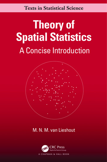
Theory of SpatialStatisticsA Concise Introduction
Theory of SpatialStatisticsA Concise IntroductionM.N.M. van Lieshout
CRC PressTaylor & Francis Group6000 Broken Sound Parkway NW, Suite 300Boca Raton, FL 33487-2742⃝c 2019 by Taylor & Francis Group, LLCCRC Press is an imprint of Taylor & Francis Group, an Informa businessNo claim to original U.S. Government worksPrinted on acid-free paperInternational Standard Book Number-13: 978-0-367-14642-9 (Hardback)978-0-367-14639-9 (Paperback)This book contains information obtained from authentic and highly regarded sources. Reasonable efforts have been made to publish reliable data and information, but the authorand publisher cannot assume responsibility for the validity of all materials or the consequences of their use. The authors and publishers have attempted to trace the copyrightholders of all material reproduced in this publication and apologize to copyright holders ifpermission to publish in this form has not been obtained. If any copyright material has notbeen acknowledged please write and let us know so we may rectify in any future reprint.Except as permitted under U.S. Copyright Law, no part of this book may be reprinted,reproduced, transmitted, or utilized in any form by any electronic, mechanical, or othermeans, now known or hereafter invented, including photocopying, microfilming, and recording, or in any information storage or retrieval system, without written permission from thepublishers.For permission to photocopy or use material electronically from this work, please accesswww.copyright.com (http://www.copyright.com/) or contact the Copyright Clearance Center, Inc. (CCC), 222 Rosewood Drive, Danvers, MA 01923, 978-750-8400. CCC is a notfor-profit organization that provides licenses and registration for a variety of users. Fororganizations that have been granted a photocopy license by the CCC, a separate systemof payment has been arranged.Trademark Notice: Product or corporate names may be trademarks or registered trademarks, and are used only for identification and explanation without intent to infringe.Library of Congress Cataloging-in-Publication DataNames: van Lieshout, M. N. M., author.Title: Theory of spatial statistics : a concise introduction / by M.N.M. vanLieshout.Description: Boca Raton, Florida : CRC Press, 2019. Includes bibliographical references and index.Identifiers: LCCN 2018052975 ISBN 9780367146429 (hardback : alk.paper) ISBN 9780367146399 (pbk. : alk. paper) ISBN 9780429052866(e-book)Subjects: LCSH: Spatial analysis (Statistics)Classification: LCC QA278.2 .V36 2019 DDC 519.5/35- -dc23LC record available at https://lccn.loc.gov/2018052975Visit the Taylor & Francis Web site athttp://www.taylorandfrancis.comand the CRC Press Web site athttp://www.crcpress.com
To Catharina Johanna Schoenmakers.
ContentsPrefacexiAuthorxiiiChapter1 ! Introduction11.1GRIDDED DATA11.2AREAL UNIT DATA31.3MAPPED POINT PATTERN DATA41.4PLAN OF THE BOOK6Chapter2 ! Random field modelling and interpolation92.1RANDOM FIELDS92.2GAUSSIAN RANDOM FIELDS112.3STATIONARITY CONCEPTS132.4CONSTRUCTION OF COVARIANCE FUNCTIONS162.5PROOF OF BOCHNER’S THEOREM202.6THE SEMI-VARIOGRAM232.7SIMPLE KRIGING262.8BAYES ESTIMATOR282.9ORDINARY KRIGING292.10 UNIVERSAL KRIGING322.11 WORKED EXAMPLES WITH R342.12 EXERCISES422.13 POINTERS TO THE LITERATURE46vii
viii ! ContentsChapter3 ! Models and inference for areal unit data493.1DISCRETE RANDOM FIELDS493.2GAUSSIAN AUTOREGRESSION MODELS523.3GIBBS STATES553.4MARKOV RANDOM FIELDS593.5INFERENCE FOR AREAL UNIT MODELS623.6MARKOV CHAIN MONTE CARLO SIMULATION673.7HIERARCHICAL MODELLING703.7.1Image segmentation703.7.2Disease mapping733.7.3Synthesis753.8WORKED EXAMPLES WITH R763.9EXERCISES843.10 POINTERS TO THE LITERATUREChapter4 ! Spatial point processes88934.1POINT PROCESSES ON EUCLIDEAN SPACES934.2THE POISSON PROCESS964.3MOMENT MEASURES984.4STATIONARITY CONCEPTS AND PRODUCTDENSITIES1004.5FINITE POINT PROCESSES1044.6THE PAPANGELOU CONDITIONAL INTENSITY1084.7MARKOV POINT PROCESSES1104.8LIKELIHOOD INFERENCE FOR POISSONPROCESSES112INFERENCE FOR FINITE POINT PROCESSES1144.94.10 COX PROCESSES1174.10.1Cluster processes1184.10.2Log-Gaussian Cox processes1204.10.3Minimum contrast estimation121
Contents ! ix4.11 HIERARCHICAL MODELLING1234.12 WORKED EXAMPLES WITH R1264.13 EXERCISES1344.14 POINTERS TO THE LITERATURE137Appendix: Solutions to theoretical exercises143Index167
PrefaceToday, much information reaches us in graphical form. From a mathematical point of view, such data may be divided into various classes,each having its own salient characteristics. For instance, in classical geostatistics, some spatially varying variable is observed at a given numberof fixed locations and one is interested in its value at locations whereit was not observed. One might think of the prediction of ore contentin the soil based on measurements at some conveniently placed boreholes or the construction of air pollution maps based on gauge data.In other cases, due to technical constraints or for privacy reasons, datais collected in aggregated form as region counts or as a discrete image.Typical examples include satellite imagery, tomographic scans, diseasemaps or yields in agricultural field trials. In this case, the objective isoften spatial smoothing or sharpening rather than prediction. Finally,data may consist of a set of objects or phenomena tied to random spatial locations and the prime interest is in the geometrical arrangementof the set, for instance in the study of earthquakes or of cellular patternsseen under a microscope.The statistical analysis of spatial data merits treatment as a separatetopic, as it is different from ‘classical’ statistical data in a number ofaspects. Typically, only a single observation is available, so that artificialreplication in the form of an appropriate stationarity assumption is calledfor. Also the size of images, or the number of objects in a spatial pattern,is typically large and, moreover, there may be interactions at variousscales. Hence a conditional or hierarchical specification is useful, oftenin combination with Monte Carlo methods.This book will describe the mathematical foundations for each ofthe data classes mentioned above, present some models and discuss statistical inference. Each chapter first presents the theory which is thenapplied to illustrative examples using an open source R-package, listssome exercises and concludes with pointers to the literature. The prerequisites consist of maturity in probability and statistics at the levelexpected of a graduate student in mathematics, engineering or statistics.xi
xii ! PrefaceIndeed, the contents grew out of lectures in the Dutch graduate school‘Mastermath’ and are suitable for a semester long introduction. Thosewishing to learn more are referred to the excellent monographs by Cressie(Wiley, 2015), by Banerjee, Carlin and Gelfand (CRC, 2004) and byGaetan and Guyon (Springer, 2010) or to the exhaustive Handbook ofSpatial Statistics (CRC, 2010).In closing, I would like to express my gratitude to the studentswho attended my ‘Mastermath’ courses for useful feedback, to the staffat Taylor and Francis, especially to Rob Calver, for their support, tothree anonymous reviewers for constructive suggestions and to ChristophHofer–Temmel for a careful reading of the manuscript.Marie-Colette van LieshoutAmsterdam, September 2018
AuthorM.N.M. van Lieshout is a senior researcher at the Centre for Mathematics and Computer Science (CWI) in Amsterdam, The Netherlands,and holds a chair in spatial stochastics at the University of Twente.xiii
CHAPTER1IntroductionThe topic of these lecture notes is modelling and inference for spatialdata. Such data, by definition, involve measurements at some spatiallocations, but can take many forms depending on the stochastic mechanism that generated the data, on the type of measurement and on thechoice of the spatial locations.Ideally, the feature of interest is measured at every location in someappropriate region, usually a bounded subset of the plane. From a mathematical point of view, such a situation can be described by a randomfield indexed by the region. In practice, however, it is not possible toconsider infinitely many locations. Additionally, there may be physical,administrative, social or economic reasons for limiting the number ofsampling locations or for storing measurements in aggregated form overareal units. The locations may even be random, so that, in mathematicalterms, they constitute a point process.In the next three sections, we will present some typical examplesto motivate the more mathematical treatment in subsequent chapters.Suggestions for statistical inference will also be given, but note that theseshould be taken as an indication. Indeed, any pertinent analysis shouldtake into account the data collection process, the specific context and thescientific question or goal that prompted data collection in the first place.1.1GRIDDED DATAFigure 1.1 shows 208 coal ash core samples collected on a grid in theRobena Mine in Greene County, Pennsylvania. The diameters of thediscs are proportional to the percentage of coal ash at the sampled locations. The data can be found in a report by Gomez and Hazen [1] and1
2 ! Introduction78.969.78510.56717.61Percentage of coal ash sampled on a grid in the Robena Minein Greene County, Pennsylvania.Figure 1.1were prepared for R by E. Pebesma using a digital version at a websitemaintained by D. Zimmerman.A mining engineer might be interested in knowing basic summarystatistics, including the first and second moments of the sample. Next,with model building in mind, he could ask himself whether the datacould have come from a normal distribution, possibly after discardingsome outliers, and if not, whether they are multi-modal or skewed. Suchquestions could be addressed by elementary tools including histograms,quantiles, boxplots and Q-Q plots.On a higher conceptual level, the mining company could also beinterested in local outliers, measured percentages that are markedly different from those around them, or in trends that could indicate goodplaces to concentrate future mining efforts. Indications of these can befound by applying the elementary statistics across rows or columns. Forinstance, consideration of the mean across columns suggests that thereis a decreasing trend in the percentage of coal ash from left to right. It
Areal unit data ! 3would be of interest to quantify how strongly correlated measurementsat adjacent sampling locations are too.Another striking feature of Figure 1.1 is that there are holes in thesampling grid, for example in the seventh row from above and in thesixth one from below. Therefore, when the mining engineer has found andvalidated a reasonable model that accounts for both the global trendsand the local dependencies in the data, he could proceed to try and fillin the gaps, in other words, to estimate the percentage of coal ash atmissing grid points based on the sampled percentages. Such a spatialinterpolation procedure is called kriging in honour of the South-Africanstatistician and mining engineer D.G. Krige, one of the pioneers of whatis now known as geostatistics.1.2AREAL UNIT DATAThe top-most panel of Figure 1.2 shows a graphical representation ofthe total number of deaths from Sudden Infant Death Syndrome (SIDS)in 1974 for each of the 100 counties in North Carolina. These data werecollected by the state’s public health statistics branch and analysed in[2]. More precisely, the counts were binned in five colour-coded intervals,where darker colours correspond to higher counts.From the picture it is clear that the centroids of the counties do notlie on a regular grid. The sizes and shapes of the counties vary and canbe quite irregular. Moreover, the recorded counts are not tied to a precise location but tallied up county-wise. This kind of accumulation overadministrative units is usual for privacy-sensitive data in, for instance,the crime or public health domains.A public health official could be interested in spatial patterns. Indeed,the original research question in [2] was whether or not there are clustersof counties with a high incidence of SIDS. However, death counts bythemselves are quite meaningless without an indication of the populationat risk. For this purpose, Symons, Grimson and Yuan [3] asked the NorthCarolina public health statistics branch for the counts of live births ineach county during the same year 1974. These are shown in the lowerpanel of Figure 1.2.Presented with the two pictures, our public health official might lookfor areas where the SIDS counts are higher than what would be expectedbased on the number of live births in the area. Such areas would beprime targets for an information campaign or a quest for factors specificto those areas that could explain the outlier. For the data at hand, whencomparing counties at the north-east and the north-west with similar
4 ! IntroductionNumbers of cases of Sudden Infant Death Syndrome (top)and live births (bottom) during 1974 accumulated per county in NorthCarolina. The death counts are binned in five classes with breaks at5, 10, 15 and 20, the live birth counts in six classes with breaks at 1000,2000, 3000, 4000 and 5000. Darker colours correspond to higher counts.Figure 1.2birth numbers, it is clear that there is a higher SIDS rate in the northeast. Note that there are also counties in the centre of the state with ahigh number of births but a rather low SIDS incidence. Other outlierscan be identified using classic boxplots and quantile techniques on therates of SIDS compared to live births.Such an analysis, however, ignores the fact that the county bordersare purely administrative and disease patterns are unlikely to follow.Moreover, rates in counties with many births are likely to be more stablethan those with few. On a higher conceptual level, the public healthauthority may therefore wish for a model that explicitly accounts forlarge scale variations in expected rates and their associated variances aswell as for local dependencies between adjacent counties.1.3MAPPED POINT PATTERN DATAFigure 1.3 shows a mapped pattern consisting of 3, 605 Beilschmiediatrees in a rectangular stand of tropical rain forest at Barro Colorado
Mapped point pattern data ! 5Top: positions of Beilschmiedia trees in a 1,000 by 500 metrestand in Barro Colorado Island, Panama. Bottom: norm of elevation (inmetres) gradient in the stand.Figure 1.3Island, Panama. These data were prepared for R by R. Waagepetersenand taken from a larger data set described in [4].We will only be interested in maps where the mechanism that generated the points is of interest. For instance, since the map of centroids ofthe North Carolina counties discussed in the previous section is purelyartificial and has no bearing on the abundance of SIDS cases, there is nopoint in studying it. For genuine mapped point pattern data, researchquestions tend to focus on the arrangement of the points, in particular,on trends and interactions.Returning to Figure 1.3, it is clear at first glance that the trees arenot distributed over the plot in a uniform way. Rather, they seem tobe concentrated in specific regions. Possible explanations could includelocal differences in soil quality or the availability of nutrients, differencesin the terrain, or traces of a planting scheme. To quantify and test nonhomogeneity, the forester may use quadrats, that is, a partition of thestand in disjoint spatial bins, and apply classical statistical dispersiontests to the quadrat counts. It might also be of interest to test whetherthe counts follow a Poisson distribution.
6 ! IntroductionSince Barro Colorado island has been studied extensively over thepast century, a lot is known about the terrain. The image in the lowermost panel of Figure 1.3 displays the norm of the elevation gradient.Visually, it seems that a steep gradient aligns well with a high treeintensity, a correlation that the forester may be interested in quantifyingby means of a spatial generalised linear regression model.The steepness of the terrain is only one factor in explaining themapped pattern. A cluster in the left part of the stand, for example,is rich in trees, even though the terrain there is not steep at all. Additionally, there could be interaction between the trees due to competitionfor nutrients or sunlight or because of seed dispersion patterns that theforester may try to capture in a model.Finally note that additional measurements might be taken at eachtree location, for example the number of stems, the size of the crown orthe diameter at breast height, but we will not pursue this topic further.1.4 PLAN OF THE BOOKChapter 2 is devoted to gridded data such as the coal ash measurementsdisplayed in Figure 1.1. The mathematical definition of a random field isgiven before specialising to Gaussian random fields. Such random fieldsare convenient to work with since their distribution is fully described bythe mean and covariance functions. Next, various types of stationarityare discussed and shown to be equivalent for Gaussian random fields.The celebrated Bochner theorem provides a spectral representation forcontinuous covariance functions.The second part of the chapter is dedicated to spatial interpolation.First, the semi-variogram and its empirical counterpart are introducedto quantify the local interaction structure in the data. A simple krigingprocedure is developed that is appropriate when both the mean and thesemi-variogram are known explicitly. It is shown that this procedure reduces to a Bayes estimator when the random field is Gaussian. In thelast sections of the chapter, the strong assumptions on mean and semivariogram are relaxed. More precisely, ordinary kriging is the name givento spatial interpolation when the mean is constant but unknown. Universal kriging is apt when explanatory variables are available to definea spatial regression for the mean.Chapter 3 is concerned with areal unit data such as the infant deathcounts shown in Figure 1.2. Special attention is given to autoregressionmodels, including Gaussian and logistic ones. It is shown that, provided
Plan of the book ! 7a positivity condition holds, the distribution of such models is fully described by their local characteristics, that is, by the family of the conditional distributions of the measurement at each areal unit given those atother units. When these local characteristics are truly local in the sensethat they depend only on the neighbours of the areal unit of interest,the random field is said to be Markov. Using the theory of Gibbs states,it is proved that the joint probability density of a Markov random fieldcan be factorised in interaction functions on sets of mutual neighbours.The second part of the chapter is devoted to statistical inference,in particular estimation of the model parameters. First, the maximumlikelihood equations are derived for a Gaussian autoregression model.For most other models, the likelihood is available only up to a parameter dependent normalisation constant. Several techniques are discussed,including maximum pseudo-likelihood and Monte Carlo maximum likelihood estimation. The chapter closes with two examples of hierarchicalmodelling and inference, image segmentation and disease mapping.The last chapter, Chapter 4, features mapped point pattern datasuch as the map of trees in Figure 1.3. The formal definition of a pointprocess is given before specialising to Poisson processes. These processesare convenient to work with because of the lack of interaction betweentheir points, and the fact that their distribution is fully described by theintensity function. Next, the moment measures and associated productdensities are defined for general point processes, together with their empirical counterparts. Various concepts of stationarity are also discussed.The remainder of the chapter is restricted to finite point processes.Following similar lines as those laid out in Chapter 3, a family of conditional distributions is defined on which a Markov property can be basedand a factorisation of the joint probability density in terms of interaction functions defined on sets of mutual neighbours is seen to hold. Amaximum likelihood theory is developed for Poisson processes, whilstthe maximum pseudo-likelihood and Monte Carlo maximum likelihoodmethods apply more generally. Minimum contrast techniques can be usedfor point processes, including Cox and cluster processes, for which thelikelihood is intractable. An application to cluster centre detection concludes the chapter.Each chapter also contains worked examples and exercises to illustrate, complement and bring the theory into practice. In order to makethe book suitable for self-study, solutions to selected exercises are collected in an appendix. The chapters close with pointers to the original
8 ! Introductionsources of the results, in so far as it was possible to trace them, and tomore specialised and elaborate textbooks for further study.The calculations in this book were done using the R-language, a free,open source implementation of the S programming language created byJ.M. Chambers [5]. R was created in the 1990s by R. Ihaka and R.Gentleman and is being developed by the R Development Core Teamcurrently consisting of some twenty people. For an introduction, we referto [6]. An attractive feature of the R-project is that it comes with a greatmany state of the art packages contributed by prominent researchers.The current list of packages is available at the site cran.r-project.org.A bit of a warning, though. Packages come with absolutely no warranty!Of course, it is also possible to write one’s own functions and to loadC-code.REFERENCES[1]M. Gomez and K. Hazen (1970). Evaluating sulfur and ash distribution in coalseams by statistical response surface regression analysis. U.S. Bureau ofMines Report RI 7377.[2]D. Atkinson (1978). Epidemiology of sudden infant death in North Carolina: Do cases tend to cluster? North Carolina Department of HumanResources, Division of Health Services Public Health Statistics BranchStudy 16.[3]M.J. Symons, R.C. Grimson and Y.C. Yuan (1983). Clustering of rare events.Biometrics 39(1):193–205.[4]S.P. Hubbell and R.B. Foster (1983). Diversity of canopy trees in neotropicalforest and implications for conservation. In: Tropical Rain Forest: Ecologyand Management. Edited by S. Sutton, T. Whitmore and A. Chadwick.Oxford: Blackwell.[5]R.A. Becker, J.M. Chambers and A.R. Wilks (1988). The New S Language.Pacific Grove, California: Wadsworth & Brooks/Cole.[6]P. Dalgaard (2008). Introductory Statistics with R (2nd edition). New York:Springer-Verlag.
CHAPTER2Random field modellingand interpolation2.1RANDOM FIELDSClimate or environmental data are often presented in the form of a map,for example the maximum temperatures on a given day in a country,the concentrations of some pollutant in a city or the mineral content insoil. In mathematical terms, such maps can be described as realisationsfrom a random field, that is, an ensemble of random quantities indexedby points in a region of interest.Definition 2.1 A random field is a family X (Xt )t T of randomvariables Xt that are defined on the same probability space and indexedby t in a subset T of Rd .Let us consider a finite set t1 , . . . , tn T of index values. Then therandom vector (Xt1 , . . . , Xtn )′ has a well-defined probability distribution that is completely determined by its joint cumulative distributionfunctionFt1 ,.,tn (x1 , . . . , xn ) P(Xt1 x1 ; · · · ; Xtn xn ),where xi R for i 1, . . . , n. The ensemble of all such joint cumulativedistribution functions with n ranging through the natural numbers andt1 , . . . , tn through T constitute the finite dimensional distributions orfidi’s of X. Together, they uniquely define the probability distributionof X.The proof relies on Kolmogorov’s consistency theorem which statesthe following. Suppose that for every finite collection t1 , . . . , tn , we have9
10 ! Random field modelling and interpolationa probability measure µt1 ,.,tn on Rn with joint cumulative distributionfunction Ft1 ,.,tn . If this family of fidi’s is symmetric in the sense thatFtπ(1) ,.,tπ(n) (xπ(1) , . . . , xπ(n) ) Ft1 ,.,tn (x1 , . . . , xn )for all n N, all x1 , . . . , xn R, all t1 , . . . , tn T and all permutationsπ of (1, . . . , n), and consistent in the sense thatlim Ft1 ,.,tn (x1 , . . . , xn ) Ft1 ,.,tn 1 (x1 , . . . , xn 1 ),xn for all n N, all x1 , . . . , xn 1 R and all t1 , . . . , tn T , then thereexists a random field X whose fidi’s coincide with those in F .In summary, in order to define a random field model, one must specifythe joint distribution of (Xt1 , . . . , Xtn )′ for all choices of n and t1 , . . . , tnin a consistent way. In the next section, we will assume that these jointdistributions are normal, and show that in that case it suffices to specifya mean and covariance function. For this reason, Gaussian models arewidely used in practice. Alternative modelling strategies may be basedon transformations, linear models, series expansions or deterministic orstochastic partitions of T , of which we present a few simple examplesbelow.Example 2.1 Fix n N and consider a partition A1 , . . . , An of T . Moreprecisely, the Ai are non-empty, disjoint sets whose union is equal to T .Let (Z1 , . . . , Zn )′ be a random n-vector and writeXt n!i 1Zi 1{t Ai }for all t T . In other words, the random surface defined by X is flaton each partition element Ai . The value set of the Zi may be finite,countable or a subset of R. In all cases, Xt is a linear combination ofrandom variables and therefore a random variable itself.Example 2.2 Fix n N and let fi : T R, i 1, . . . , n, be a set offunctions. Let (Z1 , . . . , Zn )′ be a real-valued random n-vector and writeXt n!i 1Zi fi (t),t T.Then Xt is a well-defined random variable. The fi may, for example, beharmonic or polynomial base functions, or express some spatial characteristic of interest.
Gaussian random fields ! 11One may also apply transformations to a random field to obtain newones.Example 2.3 Let X (Xt )t T be a random field and φ : R R ameasurable function. Then φ(X) (φ(Xt ))t T is also a random field.Note that the supports of the random variables Xt and φ(Xt ) may differ.The transformation φ : x exp(x), for instance, ensures that φ(Xt )takes positive values.2.2GAUSSIAN RANDOM FIELDSRecall that a random variable is normally or Gaussian distributed if ithas probability density function"#(x µ)21f (x) exp ,2σ 2σ(2π)1/2x R,with σ 2 0 or if it takes the value µ with probability one, in which caseσ 2 0. The constant µ R is the mean, σ 2 the variance.Similarly, a random vector X (X1 , . . . , Xn )′ has a multivariatenormal distribution with mean vector m (EX1 , . . . , EXn )′ Rn andn n covariance matrix Σ with entries Σij Cov(Xi , Xj ) if any linear combination a′ X ni 1 ai Xi , a Rn , is normally distributed.The normal distribution plays a central role in classical statistics. Ina spatial context, we need the following analogue.Definition 2.2 The family X (Xt )t T indexed by T Rd is a Gaussian random field if for any finite set t1 , . . . , tn of indices the randomvector (Xt1 , . . . , Xtn )′ has a multivariate normal distribution.By the definition of multivariate normality, an equivalent charac terisation is that any finite linear combination ni 1 ai Xti is normallydistributed.The finite dimensional distributions involve two parameters, themean vector and the covariance matrix. The entries of the latter areCov(Xti , Xtj ), i, j 1, . . . , n. Define the functionsm : T R;andρ : T T R;m(t) EXtρ(s, t) Cov(Xs , Xt ).
12 ! Random field modelling and interpolationThey are called the mean and covariance function of X. If we know mand ρ, we know the distributions of all (Xt1 , . . . , Xtn )′ , t1 , . . . , tn T .However, not every function from T T to R is a proper covariancefunction.Example 2.4 Examples of proper covariance functions include the following.1. The choices T R [0, ), m 0 andρ(s, t) min(s, t)define a Brownian motion.2. For m 0, β 0, andρ(s, t) 1exp ( β t s ) ,2βs, t Rd ,we obtain an Ornstein–Uhlenbeck process. The function ρ is alternatively known as an exponential covariance function.3. For β, σ 2 0, the function%&ρ(s, t) σ 2 exp β t s 2 ,is the Gaussian covariance function.s, t Rd ,4. Periodicities are taken into account by the covariance functionρ(s, t) σ 2 sinc(β t s ),s, t Rd ,for β, σ 2 0 defined in terms of the sine cardinal functionsinc(x) sin(x)/x for x ̸ 0 and 1 otherwise. Note that the correlations are alternately positive and negative, and that their absolutevalue decreases in the spatial lag t s .Proposition 2.1 The function ρ : T T R, T Rd , is the covariance function of a Gaussian random field if and only if ρ is non-negativedefinite, that is, for any t1 , . . . , tn , n N, the matrix (ρ(ti , tj ))ni,j 1 isnon-negative definite.
Stationarity concepts ! 13In other words, for any finite set t1 , . . . , tn , the matrix (ρ(ti , tj ))ni,j 1should be symmetric and satisfy the following property: for any a Rn ,nn !!i 1 j 1ai ρ(ti , tj )aj 0.Proof: “ ” Since (ρ(ti , tj ))ni,j 1 is the covariance matrix of (Xt1 , . . . ,Xtn )′ , it is non-negative definite.“ ” Apply Kolmogorov’s consistency theorem. To do so, we needto check the consistency of the fidi’s. Define µt1 ,.,tn to be a multivariate normal with covariance matrix Σ(t1 , . . . , tn ) having entries ρ(ti , tj ).By assumption, Σ(t1 , . . . , tn ) is non-negative definite so that µt1 ,.,tn iswell-defined. The µt1 ,.,tn are also consistent since they are symmetricand the marginals of normals are normal with the marginal
Printed on acid-free paper International Standard Book Number-13: 978-0-367-14642-9 (Hardback) 978-0-367-14639-9 (Paperback) This book contains information obtained from authentic and highly regarded sources. Rea-sonable efforts have been made