Transcription
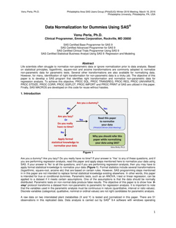
Venu Perla, Ph.D.Philadelphia Area SAS Users Group (PhilaSUG) Winter 2016 Meeting; March 16, 2016Philadelphia University, Philadelphia, PA, USAData Normalization for Dummies Using SAS Venu Perla, Ph.D.Clinical Programmer, Emmes Corporation, Rockville, MD 20850SAS Certified Base Programmer for SAS 9SAS Certified Advanced Programmer for SAS 9SAS Certified Clinical Trials Programmer Using SAS 9SAS Certified Statistical Business Analyst Using SAS 9: Regression and ModelingAbstractLife scientists often struggle to normalize non-parametric data or ignore normalization prior to data analysis. Basedon statistical principles, logarithmic, square-root and arcsine transformations are commonly adopted to normalizenon-parametric data for parametric tests. Several other transformations are also available for normalizing data.However, for many, identification of right transformation for non-parametric data is a tricky job. The objective of thispaper is to develop a SAS program that identifies right transformation and normalize non-parametric data forregression analysis. To achieve this objective, PROC SQL, PROC TRANSREG, PROC REG, PROC UNIVARIATE,PROC STDIZE, PROC CORR, PROC SGPLOT, PROC IMPORT and PROC PRINT of SAS are utilized in this paper.Finally, SAS MACROS are developed on this code for reuse without hassles.1. IntroductionFigure 1Are you a dummy? Are you lazy? Do you really have no time? If your answer is ‘Yes’ to any of these questions, and ifyou are performing regression analysis, read this paper and apply steps mentioned here to normalize your data usingSAS. If your answer is ‘No’ to all the questions, and if you are performing regression analysis, then you may have toapply formal statistical knowledge to normalize your data (Figure 1). Formal statistics include several transformations(logarithmic, square-root, arcsine etc) that are based on certain rules. However, SAS programming steps mentionedin in this paper are not intended to replace formal statistical knowledge existing elsewhere. In other words, this paperis intended for true or conditional dummies. Parametric tests, such as an ANOVA, t-test or linear regression, can beapplied to a dataset if it meets certain assumptions. One of the assumptions is that the data should be normallydistributed. Parametric tests on non-normal data produce false results. The objective of this paper is to show how ‘6step’ protocol transforms a dataset from non-parametric to parametric for regression analysis. It is important to notethat the variables used in the parametric analysis must be continuous in nature (quantitative, interval or ratio values).Discrete variables (categorical, qualitative, nominal or ordinal values) are not right candidates for parametric analysis.A raw data on two interrelated plant metabolites (X and Y) is tested and normalized in this paper. There are 51 observations in this replicated data. Data analysis is carried out by SAS 9.4 software with windows operating1
Venu Perla, Ph.D.Philadelphia Area SAS Users Group (PhilaSUG) Winter 2016 Meeting; March 16, 2016Philadelphia University, Philadelphia, PA, USA system. Data used in this paper is imported from a sheet (XY Data) of Microsoft Office Excel 97-2003 file (data1.xls)(see XY Data in Appendix). PROC IMPORT is utilized to import ‘XY Data’ and renamed it as ‘HEALTH’ (Table 1).%let path C:\Users\Perla\Desktop\;title "Importing data from excel";proc import file "&path.data1.xls"out health replacedbms xls;sheet XY Data;getnames yes;run;title "Checking imported data";proc print data health;run;For importing XY Data, macro EXCEL IMPORT is developed on above code (see Appendix). This macro can beutilized in future for analysis of similar data by running following code:%excel import (excel file , excel sheet , dataset );2. Data NormalizationAfter importing data into SAS, a ‘6-step’ protocol for normalization of data for regression analysis using SAS ispresented in Figure 2. Programming aspects of each step are also discussed in this section.Step 1: Check Scatter Plot and Correlation MatrixRelationship between X- and Y-variables can be visualized using PROC SGPLOT and PROC CORR.ods graphics on;title "Scatter plot of X and Y";proc sgplot data health;scatter x x y y;run;title "Correlation between X and Y";proc corr data health;var x y;run;ods graphics off;Scatter plot of X and Y indicates that there is no clear relationship between these two variables (Figure 3). Results onPearson correlation coefficients indicate a weak correlation between X- and Y-variables (Table 2).2
Venu Perla, Ph.D.Philadelphia Area SAS Users Group (PhilaSUG) Winter 2016 Meeting; March 16, 2016Philadelphia University, Philadelphia, PA, USAFigure 2Figure 3Table 2Above code is utilized to develop a macro, ‘SCATTER CORR’ (See Appendix). This macro can be utilized in futurefor analysis of similar data by running following code:%scatter corr (dataset , xvar , yvar );3
Venu Perla, Ph.D.Philadelphia Area SAS Users Group (PhilaSUG) Winter 2016 Meeting; March 16, 2016Philadelphia University, Philadelphia, PA, USAStep 2: Perform Regression Analysis and Normality TestsThere is an indication of a weak correlation between X and Y (Pearson correlation coefficient: 0.35). Further analysisis carried out on this raw data using PROC REG and PROC UNIVARIATE. LACKFIT option of MODEL statement inPROC REG determines whether this linear model is a good fit for this replicated data or not? Residual analysis andndnormality tests are carried out using PROC UNIVARIATE with NORMAL option. If data is normal after 2 step, nofurther steps are required to execute to normalize the data.ODS graphics on;title "Regression analysis";proc reg data health plots(only) diagnostics (unpack);model y x/lackfit;output out mdlres r resid;run;ODS graphics off;proc univariate data mdlres normal;var resid;run;Analysis of variance indicates that LACK OF FIT for the linear model is significant (Table 3). This suggests thatfurther in-depth analysis has to be carried out on this raw data before rejecting the model.2Parameter estimates and adjusted R value for the raw data are provided in Table 4A and 4B, respectively. Adjusted2R value is negligible (0.11).Distribution of residuals for Y is not normal for the raw data (Figure 4).4
Venu Perla, Ph.D.Philadelphia Area SAS Users Group (PhilaSUG) Winter 2016 Meeting; March 16, 2016Philadelphia University, Philadelphia, PA, USAFigure 4Furthermore, significant p values for four tests of normality are the true testimony of non-normal distribution of data(Table 5).Table 5Above code is utilized to develop a macro ‘REG NORMALITY’ (See Appendix). This macro can be utilized in futurefor analysis of similar data by running following code:%reg normality (dataset health, xvar x, yvar y);Step 3: Transform Data into Non-zero and Non-negative DataBox-Cox power transformation can be adopted to normalize this raw data. Data should be converted to non-zero andnon-negative values before testing for Box-Cox power transformation. Following code transforms X- and Y-variablesinto non-zero and/or non- negative variables only when ‘0’ or negative values are encountered in the data.PROC SQL is used to transform X- and Y-variable data into non-zero and non-negative data. Table HEALTH COX iscreated from dataset HEALTH in this procedure. Proc SQL reproduced original data as there are no zeros and nonegative values (Table 6).title "Transforming X and Y values into non-zero and non-negative values";proc sql;create table health cox asselect casewhen min(x) 0 then (-(min(x)) x 1)else xend as X,casewhen min(y) 0 then (-(min(y)) y 1)else yend as Yfrom health;quit;proc print data health cox;5
Venu Perla, Ph.D.Philadelphia Area SAS Users Group (PhilaSUG) Winter 2016 Meeting; March 16, 2016Philadelphia University, Philadelphia, PA, USArun;Table 6Macro ‘TRANSFORM ZERO NEG’ is developed for above PROC SQL code (See Appendix). This macro can beinvoked in future by following statement:%transform zero neg (dataset ,xvar ,yvar ,pre trans dataset );Step 4: Perform Box-Cox Power TransformationBox-Cox power transformation on non-zero and non-negative data is performed using PROC TRANSREG with ODSGRAPHICS on.title "Box-Cox power transformation: Identification of right exponent(Lambda)";ods graphics on;proc transreg data health cox;model boxcox(y) identity(x);run;ods graphics off;Above code generated Box-Cox analysis for Y (Figure 5). Selected lambda (-0.75 at 95% CI) is the exponent to beused to transform the data into normal shape.Figure 5In order to get convenient lambda value, above SAS code is executed without ODS GRAPHICS statement.proc transreg data health cox;model boxcox(y) identity(x);run;6
Venu Perla, Ph.D.Philadelphia Area SAS Users Group (PhilaSUG) Winter 2016 Meeting; March 16, 2016Philadelphia University, Philadelphia, PA, USAThis code generated best lambda, lambda with 95% confidence interval, and convenient lambda (Table 7).Convenient lambda is used for transforming Y-variable in this analysis.Table 7Macro ‘BOX COX LAMBDA’ is developed on above code (See Appendix). This macro can be utilized in future foranalysis of similar data by running following code:%box cox lambda (pre trans dataset , xvar ,yvar );PROC SQL program is used to transform Y-variable. Code for common convenient lambda values (-2, -1, -0.5, 0, 0.5,221 and 2); respective Y-transformations (1/Y , 1/Y, 1/sqrt (Y), log (Y), sqrt (Y), Y and Y ); and respective transformed-Yvariable names (neg 2 y, neg 1 y, neg half y, zero y, half y, one y, and two y) are incorporated in the program.title "Transformation of Y-values with convenient lambda";proc sql;create table health trans asselectx, y,1/(y**2) as neg 2 y,1/(y**1) as neg 1 y,1/(sqrt(y)) as neg half y,log(y) as zero y,sqrt(y) as half y,y**1 as one y,y**2 as two yfrom health cox;quit;proc print data health trans;run;PROC SQL generated ‘HEALTH TRANS’ table (Table 8). ‘neg 1 y’ is the corresponding transformed Y-variable forthe convenient lambda -1. This ‘neg 1 y’ variable is used for further analysis.7
Venu Perla, Ph.D.Philadelphia Area SAS Users Group (PhilaSUG) Winter 2016 Meeting; March 16, 2016Philadelphia University, Philadelphia, PA, USATable 8Macro ‘TRANSFORM LAMBDA’ is defined on above PROC SQL code (See Appendix). This macro can be utilizedin future for analysis of similar data by running following code:%transform lambda (pre trans dataset , xvar , yvar , trans dataset );Step 5: Standardize X-variableAfter transformation of Y-variable, in order to obtain meaningful Y-intercept, X-variable is standardized using PROCSTDIZE. Dataset ‘HEALTH2’ is generated from table ‘HEALTH TRANS’ in this procedure. OPREFIX option is usedto prefix the original X-variable name with the word, ‘Unstdized ’. On the other hand, standardized X-values arestored under X.title "Standardized X-variable after Y-transformation";proc stdize data health transoprefix Unstdizedmethod meanout health2;var x;run;proc print data health2;run;Generated dataset ‘HEALTH2’ is shown below with standardized X-variable in the last column as X (Table 9).Table 9Macro ‘STDIZE X’ is defined on above code (See Appendix). It can be invoked in future by calling followingstatement:%stdize x (trans dataset , trans stdize dataset , xvar );Step 6: Perform Regression Analysis and Normality TestsRegression analysis and normality tests are again performed on the transformed and standardized dataset‘HEALTH2’ by calling previously defined macro ‘REG NORMALITY’. Variable X is the standardized X, and ‘neg 1 y’is the transformed Y.%reg normality (dataset health2, xvar x, yvar neg 1 y);With transformed data, LACK OF FIT for linear model is turned out to be non-significant, which indicates that thelinear model is acceptable for X and Y (Table 10). Parameter estimates for intercept and X are significant (Table 11).2As compared to the raw data, adjusted R value with transformed data is improved from 0.11 to 0.53 (Table 12).8
Venu Perla, Ph.D.Philadelphia Area SAS Users Group (PhilaSUG) Winter 2016 Meeting; March 16, 2016Philadelphia University, Philadelphia, PA, USAOther results indicate that transformed data is normally distributed (Figure 6; Table 13). Non-significant p-value withKolmogorov-Smirnov normality test further confirms that data is normally distributed (Table 13).Table 10Table 11Table 12Table 139
Venu Perla, Ph.D.Philadelphia Area SAS Users Group (PhilaSUG) Winter 2016 Meeting; March 16, 2016Philadelphia University, Philadelphia, PA, USA3. Normalization Eliminates Misleading Results2Negligible positive correlation exists between X and Y in raw data (Adjusted R : 0.11). After normalization, there is a2moderate positive correlation between X and Y (Adjusted R : 0.53). In other words, normalization eliminatesmisleading results.2Raw data (non-parametric):Normalized data:Y 0.124 0.933X (Adjusted R : 0.11)2Y 1.240 – 0.514X (Adjusted R : 0.53)4. Limitations and SolutionsOutliers in a data may drastically affect normalization. Three out of four tests of normality are still significant in thisanalysis (Table 13). It indicates that there is a room for further improvement of data with respect to normalization. Ingeneral, non-parametric nature of data after step 6 indicates presence of outliers in the dataset. There is at least oneoutlier and leverage observation that is influencing the normal distribution here (Figure 7). Techniques to isolate andrescue outliers while normalizing the data were presented at the Ohio SAS Users Group Conference (Perla, 2015A),and at the Philadelphia Area SAS Users Group Fall Meeting (Perla, 2015B) (Figure 8 and 9). Another potentiallimitation for ‘6-step’ protocol is the field of study. Perhaps, ‘6-step’ protocol can be applied in any filed. However,sometimes, it may be more meaningful to adopt a transformation that is commonly used in that field of study.Figure 7Figure 8Figure 95. ConclusionsIn summary, misleading results are produced if parametric tests, such as t-test, ANOVA or linear regression, areapplied on non-parametric data. A ‘6-step’ protocol discussed in this paper is a good option for normalizing data for10
Venu Perla, Ph.D.Philadelphia Area SAS Users Group (PhilaSUG) Winter 2016 Meeting; March 16, 2016Philadelphia University, Philadelphia, PA, USAregression analysis. In the real world, outliers are the major limitation while normalizing the data. I have recentlyexplained a technique to isolate and rescue outliers while normalizing the data. Refer Perla (2005A and B) for moredetails and macro definitions.References Carpenter, Art. 2004. Carpenter’s Complete Guide to the SAS Macro Language, Second Edition, SAS Institute Inc.,Cary, NC, USA. Gupta, Sunil. 2016. Sharpening Your Advanced SAS Skills. CRC Press, Boca Raton, FL, USA. Lafler, Kirk Paul. 2013. PROC SQL: Beyond the Basics Using SAS , Second Edition, SAS Institute Inc., Cary, NC,USA. Li, Arthur. 2013. Handbook of SAS DATA Step Programming. CRC Press, Boca Raton, FL, USA. Perla, Venu. 2015A. How PROC SQL and SAS Macro Programming Made My Statistical Analysis Easy? A Case Study on Linear Regression. Ohio SAS Users Conference held on June 1, 2015 at the Kingsgate MarriottConference Center at the University of Cincinnati, Cincinnati, Ohio, USA. Available near%20Regression.pdf Perla, Venu. 2015B. A Technique to Rescue Non-parametric Outlier Data Using SAS . Philadelphia Area SASUsers Group Fall Meeting held on October 29, 2015 at the Penn State Great Valley School of GraduateProfessional Studies, Malvern, PA, USA. Available PSU/2015-Oct-Venu%20Perla-Final.pdf SAS 9.4 Product Documentation, SAS Institute Inc., Cary, NC, USA. Available ml SAS/STAT 9.3 User's Guide, SAS Institute Inc., Cary, NC, USA. Available ug/63962/HTML/default/viewer.htm#intro toc.htm SAS 9.2 Macro Language: Reference, SAS Institute Inc., Cary, NC, USA. Available lref/61885/HTML/default/viewer.htm#titlepage.htm SAS 9.3 SQL Procedure User’s Guide, SAS Institute Inc., Cary, NC, USA. Available nowledgments I would like to thank the organizers for giving me an opportunity to present this paper at the Philadelphia SAS UsersGroup Winter Meeting on March 16, 2016 at the Tuttleman Center, Philadelphia University, Philadelphia, PA, USA.Trademark CitationsSAS and all other SAS Institute Inc. product or service names are registered trademarks or trademarks of SASInstitute Inc. in the USA and other countries. indicates USA registration.Author BiographyVenu Perla, Ph.D. is a SAS Certified Advanced Programmer, Clinical Programmer andStatistical Business Analyst for SAS 9. Dr. Perla is also a biomedical researcher withabout 14 years of research and teaching experience in an academic environment. Heserved the Purdue University, Oregon Health & Science University, Colorado StateUniversity, West Virginia State University R&D Corporation, Kerala Agricultural University(India) and Mangalayatan University (India) at different capacities. Dr. Perla haspublished 15 scientific papers and 2 book chapters, obtained 1 international patent onorthopaedic implant device, gave 9 talks and presented 18 posters at national andinternational scientific conferences in his professional career. Dr. Perla was invited toserve as an editorial board member for several national and international scientificjournals. He was trained in clinical trials and clinical data management. Currently, he is actively employing SAS programming techniques in clinical data analysis.Contact InformationPhone (Cell): (304) 545-5705Email: venuperla@yahoo.comvperla@emmes.comLinkedIn: 11
Venu Perla, Ph.D.Philadelphia Area SAS Users Group (PhilaSUG) Winter 2016 Meeting; March 16, 2016Philadelphia University, Philadelphia, PA, USAAppendixXY Data sheet of data1.xls (Microsoft Excel 97-2003 50.720.70.82.71.511.60.80.70.70.81.4112
Venu Perla, Ph.D.Philadelphia Area SAS Users Group (PhilaSUG) Winter 2016 Meeting; March 16, 2016Philadelphia University, Philadelphia, PA, USAMacro ‘EXCEL IMPORT’:Macro ‘EXCEL IMPORT’ is defined below for importing Excel files. Where, ‘EXCEL FILE ’ is name of the excel fileto be used; ‘EXCEL SHEET ’ is name of the excel sheet to be imported; and ‘DATASET ’ is name of the outputdataset. File extension and DBMS statement in the code may be modified according to the Excel version used.%macro excel import (excel file , excel sheet , dataset );title "Importing data from excel";proc import file "&path.&excel file.xls"out &dataset replacedbms xls;sheet &excel sheet;getnames yes;run;title "Dataset from imported excel data";proc print data &dataset;run;%mend excel import;This macro can be invoked by calling following code for this paper:%excel import (excel file data1, excel sheet XY Data, dataset health);Macro ‘SCATTER CORR’:Macro ‘SCATTER CORR’ is defined below . Where, ‘DATASET ’ is name of the dataset to be used for analysis; and‘XVAR ’ and ‘YVAR ’ are the names of the X- and Y-variables, respectively.%macro scatter corr (dataset , xvar , yvar );ods graphics on;title "Scatter plot of &xvar and &yvar";proc sgplot data &dataset;scatter x &xvar y &yvar;run;title "Correlation between &xvar and &yvar";proc corr data &dataset;var &xvar &yvar;run;ods graphics off;%mend scatter corr;This macro can be invoked by following statement for this paper:%scatter corr (dataset health, xvar x, yvar y);Macro ‘REG NORMALITY’:Macro ‘REG NORMALITY’ is defined below for regression analysis and normality tests. Where, ‘DATASET ’ is nameof the dataset to be used for analysis; and ‘XVAR ’ and ‘YVAR ’ are names of the X- and Y-variables, respectively.%macro reg normality (dataset ,xvar ,yvar );ODS graphics on;title "Regression analysis: Dataset &dataset";proc reg data &dataset plots(only) diagnostics (unpack);model &yvar &xvar/lackfit;output out mdlres r resid;run;13
Venu Perla, Ph.D.Philadelphia Area SAS Users Group (PhilaSUG) Winter 2016 Meeting; March 16, 2016Philadelphia University, Philadelphia, PA, USAproc univariate data mdlres normal;var resid;run;ODS graphics off;%mend reg normality;This macro can be invoked by following statement for this paper:%reg normality (dataset health, xvar x, yvar y);Macro ‘TRANSFORM ZERO NEG’:Macro ‘TRANSFORM ZERO NEG’ is defined below. Where, ‘DATASET ’ is the name of the input dataset to beused for transforming X- and Y-values; ‘XVAR ’ and ‘YVAR ’ are names of the X- and Y-variables to be transformed,respectively; and ‘PRE TRANS DATASET ’ is name of the output dataset to be created with transformed X- and Yvariables.%macro transform zero neg (dataset ,xvar ,yvar ,pre trans dataset );title "Transforming &xvar and &yvar values into non-zero and non-negativevalues";proc sql;create table &pre trans dataset asselect casewhen min(&xvar) 0 then (-(min(&xvar)) &xvar 1)else &xvarend as &xvar,casewhen min(&yvar) 0 then (-(min(&yvar)) &yvar 1)else &yvarend as &yvarfrom &dataset;quit;proc print data &pre trans dataset;run;%mend transform zero neg;This macro can be invoked by following statement for this paper:%transform zero neg(dataset health,xvar x,yvar y,pre trans dataset health cox);Macro ‘BOX COX LAMBDA’:Macro ‘BOX COX LAMBDA’ is defined below. Where, ‘PRE TRANS DATASET ’ is name of the input dataset withnon-zero and non-negative values; and ‘XVAR ’ and ‘YVAR ’ are names of the X- and Y-variables, respectively.%macro box cox lambda (pre trans dataset ,xvar ,yvar );title "Box-Cox power transformation: Identification of right exponent(Lambda)";ods graphics on;proc transreg data &pre trans dataset;model boxcox(&yvar) identity(&xvar);run;ods graphics off;proc transreg data &pre trans dataset;model boxcox(&yvar) identity(&xvar);run;%mend box cox lambda;14
Venu Perla, Ph.D.Philadelphia Area SAS Users Group (PhilaSUG) Winter 2016 Meeting; March 16, 2016Philadelphia University, Philadelphia, PA, USAThis macro can be invoked by following statement for this paper:%box cox lambda (pre trans dataset health cox, xvar x ,yvar y);Macro ‘TRANSFORM LAMBDA’:Macro ‘TRANSFORM LAMBDA’ is defined below. Where, ‘PRE TRANS DATASET ’ is name of the input datasetwith non-zero and non-negative X- and Y-values; ‘XVAR ’ and ‘YVAR ’ are names of the X- and Y-variables,respectively; and ‘TRANS DATASET ’ is name of the output dataset with transformed data.%macro transform lambda (pre trans dataset ,xvar ,yvar ,trans dataset );title "Transformation of &yvar.-values with convenient lambda";proc sql;create table &trans dataset asselect&xvar, &yvar,1/(&yvar**2) as neg 2 &yvar,1/(&yvar**1) as neg 1 &yvar,1/(sqrt(&yvar)) as neg half &yvar,log(&yvar) as zero &yvar,sqrt(&yvar) as half &yvar,&yvar**1 as one &yvar,&yvar**2 as two &yvarfrom &pre trans dataset;quit;proc print data &trans dataset;run;%mend transform lambda;This macro can be invoked by following statement for this paper:%transform lambda (pre trans dataset health cox, xvar x, yvar y,trans dataset health trans);Macro ‘STDIZE X’:Macro ‘STDIZE X’ is defined below. Where, ‘TRANS DATASET ’ is name of the input dataset;‘TRANS STDIZE DATASET ’ is name of the output dataset; and ‘XVAR ’ is name of the X-variable to bestandardized.%macro stdize x (trans dataset ,trans stdize dataset ,xvar );title "Standardized &xvar.-variable after Y-transformation";proc stdize data &trans datasetoprefix Unstdizedmethod meanout &trans stdize dataset;var &xvar;run;proc print data &trans stdize dataset;run;%mend stdize x;This macro can be invoked by following statement for this paper:%stdize x (trans dataset health trans, trans stdize dataset health2, xvar x);15
utilized in future for analysis of similar data by running following code: %excel_import (excel_file , excel_sheet , dataset ); 2. Data Normalization After importing data into SAS, a ‘6-step’ protocol for normalization of data for regression analysis using SAS is presented in Figure 2
