Transcription
TECHNICAL REPORTR-350September 2009Statistics SurveysVol. 3 (2009) 96–146ISSN: 1935-7516DOI: 10.1214/09-SS057Causal inference in statistics:An overview †‡Judea PearlComputer Science DepartmentUniversity of California, Los Angeles, CA 90095 USAe-mail: judea@cs.ucla.eduAbstract: This review presents empirical researchers with recent advancesin causal inference, and stresses the paradigmatic shifts that must be undertaken in moving from traditional statistical analysis to causal analysis ofmultivariate data. Special emphasis is placed on the assumptions that underly all causal inferences, the languages used in formulating those assumptions, the conditional nature of all causal and counterfactual claims, andthe methods that have been developed for the assessment of such claims.These advances are illustrated using a general theory of causation basedon the Structural Causal Model (SCM) described in Pearl (2000a), whichsubsumes and unifies other approaches to causation, and provides a coherent mathematical foundation for the analysis of causes and counterfactuals.In particular, the paper surveys the development of mathematical tools forinferring (from a combination of data and assumptions) answers to threetypes of causal queries: (1) queries about the effects of potential interventions, (also called “causal effects” or “policy evaluation”) (2) queries aboutprobabilities of counterfactuals, (including assessment of “regret,” “attribution” or “causes of effects”) and (3) queries about direct and indirecteffects (also known as “mediation”). Finally, the paper defines the formaland conceptual relationships between the structural and potential-outcomeframeworks and presents tools for a symbiotic analysis that uses the strongfeatures of both.Keywords and phrases: Structural equation models, confounding, graphical methods, counterfactuals, causal effects, potential-outcome, mediation,policy evaluation, causes of effects.Received September 2009.Contents12Introduction . . . . . . . . . . . . . . . . . . . . . .From association to causation . . . . . . . . . . . .2.1 The basic distinction: Coping with change . . .2.2 Formulating the basic distinction . . . . . . . .2.3 Ramifications of the basic distinction . . . . . .2.4 Two mental barriers: Untested assumptions and. . . . . . . . . . . . . . . . . . . . . . . . . . . . . . . . . . . .new notation. 97. 99. 99. 99. 100. 101 Portions of this paper are based on my book Causality (Pearl, 2000, 2nd edition 2009),and have benefited appreciably from conversations with readers, students, and colleagues.† This research was supported in parts by an ONR grant #N000-14-09-1-0665.‡ This paper was accepted by Elja Arjas, Executive Editor for the Bernoulli.96
J. Pearl/Causal inference in statistics3Structural models, diagrams, causal effects, and counterfactuals . . . .3.1 Introduction to structural equation models . . . . . . . . . . . .3.2 From linear to nonparametric models and graphs . . . . . . . . .3.2.1 Representing interventions . . . . . . . . . . . . . . . . . .3.2.2 Estimating the effect of interventions . . . . . . . . . . . .3.2.3 Causal effects from data and graphs . . . . . . . . . . . .3.3 Coping with unmeasured confounders . . . . . . . . . . . . . . .3.3.1 Covariate selection – the back-door criterion . . . . . . . .3.3.2 General control of confounding . . . . . . . . . . . . . . .3.3.3 From identification to estimation . . . . . . . . . . . . . .3.3.4 Bayesianism and causality, or where do the probabilitiescome from? . . . . . . . . . . . . . . . . . . . . . . . . . .3.4 Counterfactual analysis in structural models . . . . . . . . . . . .3.5 An example: Non-compliance in clinical trials . . . . . . . . . . .3.5.1 Defining the target quantity . . . . . . . . . . . . . . . . .3.5.2 Formulating the assumptions – Instrumental variables . .3.5.3 Bounding causal effects . . . . . . . . . . . . . . . . . . .3.5.4 Testable implications of instrumental variables . . . . . .4 The potential outcome framework . . . . . . . . . . . . . . . . . . . .4.1 The “Black-Box” missing-data paradigm . . . . . . . . . . . . . .4.2 Problem formulation and the demystification of “ignorability” . .4.3 Combining graphs and potential outcomes . . . . . . . . . . . .5 Counterfactuals at work . . . . . . . . . . . . . . . . . . . . . . . . . .5.1 Mediation: Direct and indirect effects . . . . . . . . . . . . . . . .5.1.1 Direct versus total effects: . . . . . . . . . . . . . . . . .5.1.2 Natural direct effects . . . . . . . . . . . . . . . . . . . . .5.1.3 Indirect effects and the Mediation Formula . . . . . . . .5.2 Causes of effects and probabilities of causation . . . . . . . . . .6 Conclusions . . . . . . . . . . . . . . . . . . . . . . . . . . . . . . . . .References . . . . . . . . . . . . . . . . . . . . . . . . . . . . . . . . . . . 41251261271281311321321321341351361391391. IntroductionThe questions that motivate most studies in the health, social and behavioralsciences are not associational but causal in nature. For example, what is theefficacy of a given drug in a given population? Whether data can prove anemployer guilty of hiring discrimination? What fraction of past crimes couldhave been avoided by a given policy? What was the cause of death of a givenindividual, in a specific incident? These are causal questions because they requiresome knowledge of the data-generating process; they cannot be computed fromthe data alone, nor from the distributions that govern the data.Remarkably, although much of the conceptual framework and algorithmictools needed for tackling such problems are now well established, they are hardlyknown to researchers who could put them into practical use. The main reason iseducational. Solving causal problems systematically requires certain extensions
J. Pearl/Causal inference in statistics98in the standard mathematical language of statistics, and these extensions are notgenerally emphasized in the mainstream literature and education. As a result,large segments of the statistical research community find it hard to appreciateand benefit from the many results that causal analysis has produced in the pasttwo decades. These results rest on contemporary advances in four areas:1.2.3.4.Counterfactual analysisNonparametric structural equationsGraphical modelsSymbiosis between counterfactual and graphical methods.This survey aims at making these advances more accessible to the general research community by, first, contrasting causal analysis with standard statisticalanalysis, second, presenting a unifying theory, called “structural,” within whichmost (if not all) aspects of causation can be formulated, analyzed and compared,thirdly, presenting a set of simple yet effective tools, spawned by the structuraltheory, for solving a wide variety of causal problems and, finally, demonstratinghow former approaches to causal analysis emerge as special cases of the generalstructural theory.To this end, Section 2 begins by illuminating two conceptual barriers that impede the transition from statistical to causal analysis: (i) coping with untestedassumptions and (ii) acquiring new mathematical notation. Crossing these barriers, Section 3.1 then introduces the fundamentals of the structural theoryof causation, with emphasis on the formal representation of causal assumptions, and formal definitions of causal effects, counterfactuals and joint probabilities of counterfactuals. Section 3.2 uses these modeling fundamentals torepresent interventions and develop mathematical tools for estimating causaleffects (Section 3.3) and counterfactual quantities (Section 3.4). These tools aredemonstrated by attending to the analysis of instrumental variables and theirrole in bounding treatment effects in experiments marred by noncompliance(Section 3.5).The tools described in this section permit investigators to communicate causalassumptions formally using diagrams, then inspect the diagram and1. Decide whether the assumptions made are sufficient for obtaining consistent estimates of the target quantity;2. Derive (if the answer to item 1 is affirmative) a closed-form expression forthe target quantity in terms of distributions of observed quantities; and3. Suggest (if the answer to item 1 is negative) a set of observations and experiments that, if performed, would render a consistent estimate feasible.Section 4 relates these tools to those used in the potential-outcome framework, and offers a formal mapping between the two frameworks and a symbiosis(Section 4.3) that exploits the best features of both. Finally, the benefit of thissymbiosis is demonstrated in Section 5, in which the structure-based logic ofcounterfactuals is harnessed to estimate causal quantities that cannot be defined within the paradigm of controlled randomized experiments. These includedirect and indirect effects, the effect of treatment on the treated, and ques-
J. Pearl/Causal inference in statistics99tions of attribution, i.e., whether one event can be deemed “responsible” foranother.2. From association to causation2.1. The basic distinction: Coping with changeThe aim of standard statistical analysis, typified by regression, estimation, andhypothesis testing techniques, is to assess parameters of a distribution fromsamples drawn of that distribution. With the help of such parameters, one caninfer associations among variables, estimate beliefs or probabilities of past andfuture events, as well as update those probabilities in light of new evidenceor new measurements. These tasks are managed well by standard statisticalanalysis so long as experimental conditions remain the same. Causal analysisgoes one step further; its aim is to infer not only beliefs or probabilities understatic conditions, but also the dynamics of beliefs under changing conditions,for example, changes induced by treatments or external interventions.This distinction implies that causal and associational concepts do not mix.There is nothing in the joint distribution of symptoms and diseases to tell usthat curing the former would or would not cure the latter. More generally, thereis nothing in a distribution function to tell us how that distribution would differif external conditions were to change—say from observational to experimentalsetup—because the laws of probability theory do not dictate how one propertyof a distribution ought to change when another property is modified. This information must be provided by causal assumptions which identify relationshipsthat remain invariant when external conditions change.These considerations imply that the slogan “correlation does not imply causation” can be translated into a useful principle: one cannot substantiate causalclaims from associations alone, even at the population level—behind everycausal conclusion there must lie some causal assumption that is not testablein observational studies.12.2. Formulating the basic distinctionA useful demarcation line that makes the distinction between associational andcausal concepts crisp and easy to apply, can be formulated as follows. An associational concept is any relationship that can be defined in terms of a jointdistribution of observed variables, and a causal concept is any relationship thatcannot be defined from the distribution alone. Examples of associational concepts are: correlation, regression, dependence, conditional independence, likelihood, collapsibility, propensity score, risk ratio, odds ratio, marginalization,1 The methodology of “causal discovery” (Spirtes et al. 2000; Pearl 2000a, Chapter 2) islikewise based on the causal assumption of “faithfulness” or “stability,” a problem-independentassumption that concerns relationships between the structure of a model and the data itgenerates.
J. Pearl/Causal inference in statistics100conditionalization, “controlling for,” and so on. Examples of causal concepts are:randomization, influence, effect, confounding, “holding constant,” disturbance,spurious correlation, faithfulness/stability, instrumental variables, intervention,explanation, attribution, and so on. The former can, while the latter cannot bedefined in term of distribution functions.This demarcation line is extremely useful in causal analysis for it helps investigators to trace the assumptions that are needed for substantiating varioustypes of scientific claims. Every claim invoking causal concepts must rely onsome premises that invoke such concepts; it cannot be inferred from, or evendefined in terms statistical associations alone.2.3. Ramifications of the basic distinctionThis principle has far reaching consequences that are not generally recognizedin the standard statistical literature. Many researchers, for example, are stillconvinced that confounding is solidly founded in standard, frequentist statistics, and that it can be given an associational definition saying (roughly): “U isa potential confounder for examining the effect of treatment X on outcome Ywhen both U and X and U and Y are not independent.” That this definitionand all its many variants must fail (Pearl, 2000a, Section 6.2)2 is obvious fromthe demarcation line above; if confounding were definable in terms of statisticalassociations, we would have been able to identify confounders from features ofnonexperimental data, adjust for those confounders and obtain unbiased estimates of causal effects. This would have violated our golden rule: behind anycausal conclusion there must be some causal assumption, untested in observational studies. Hence the definition must be false. Therefore, to the bitterdisappointment of generations of epidemiologist and social science researchers,confounding bias cannot be detected or corrected by statistical methods alone;one must make some judgmental assumptions regarding causal relationships inthe problem before an adjustment (e.g., by stratification) can safely correct forconfounding bias.Another ramification of the sharp distinction between associational and causalconcepts is that any mathematical approach to causal analysis must acquire newnotation for expressing causal relations – probability calculus is insufficient. Toillustrate, the syntax of probability calculus does not permit us to express thesimple fact that “symptoms do not cause diseases,” let alone draw mathematicalconclusions from such facts. All we can say is that two events are dependent—meaning that if we find one, we can expect to encounter the other, but we cannot distinguish statistical dependence, quantified by the conditional probabilityP (disease symptom) from causal dependence, for which we have no expressionin standard probability calculus. Scientists seeking to express causal relationships must therefore supplement the language of probability with a vocabulary2 For example, any intermediate variable U on a causal path from X to Y satisfies thisdefinition, without confounding the effect of X on Y .
J. Pearl/Causal inference in statistics101for causality, one in which the symbolic representation for the relation “symptoms cause disease” is distinct from the symbolic representation of “symptomsare associated with disease.”2.4. Two mental barriers: Untested assumptions and new notationThe preceding two requirements: (1) to commence causal analysis with untested,3theoretically or judgmentally based assumptions, and (2) to extend the syntaxof probability calculus, constitute the two main obstacles to the acceptance ofcausal analysis among statisticians and among professionals with traditionaltraining in statistics.Associational assumptions, even untested, are testable in principle, given sufficiently large sample and sufficiently fine measurements. Causal assumptions, incontrast, cannot be verified even in principle, unless one resorts to experimentalcontrol. This difference stands out in Bayesian analysis. Though the priors thatBayesians commonly assign to statistical parameters are untested quantities,the sensitivity to these priors tends to diminish with increasing sample size. Incontrast, sensitivity to prior causal assumptions, say that treatment does notchange gender, remains substantial regardless of sample size.This makes it doubly important that the notation we use for expressing causalassumptions be meaningful and unambiguous so that one can clearly judge theplausibility or inevitability of the assumptions articulated. Statisticians can nolonger ignore the mental representation in which scientists store experientialknowledge, since it is this representation, and the language used to access it thatdetermine the reliability of the judgments upon which the analysis so cruciallydepends.How does one recognize causal expressions in the statistical literature? Thoseversed in the potential-outcome notation (Neyman, 1923; Rubin, 1974; Holland,1988), can recognize such expressions through the subscripts that are attachedto counterfactual events and variables, e.g. Yx (u) or Zxy . (Some authors useparenthetical expressions, e.g. Y (0), Y (1), Y (x, u) or Z(x, y).) The expressionYx (u), for example, stands for the value that outcome Y would take in individual u, had treatment X been at level x. If u is chosen at random, Yx is arandom variable, and one can talk about the probability that Yx would attaina value y in the population, written P (Yx y) (see Section 4 for semantics).Alternatively, Pearl (1995a) used expressions of the form P (Y y set(X x))or P (Y y do(X x)) to denote the probability (or frequency) that event(Y y) would occur if treatment condition X x were enforced uniformlyover the population.4 Still a third notation that distinguishes causal expressionsis provided by graphical models, where the arrows convey causal directionality.53 By“untested” I mean untested using frequency data in nonexperimental studies.P (Y y do(X x)) is equivalent to P (Yx y). This is what we normally assessin a controlled experiment, with X randomized, in which the distribution of Y is estimatedfor each level x of X.5 These notational clues should be useful for detecting inadequate definitions of causalconcepts; any definition of confounding, randomization or instrumental variables that is cast in4 Clearly,
J. Pearl/Causal inference in statistics102However, few have taken seriously the textbook requirement that any introduction of new notation must entail a systematic definition of the syntax andsemantics that governs the notation. Moreover, in the bulk of the statistical literature before 2000, causal claims rarely appear in the mathematics. They surfaceonly in the verbal interpretation that investigators occasionally attach to certain associations, and in the verbal description with which investigators justifyassumptions. For example, the assumption that a covariate not be affected bya treatment, a necessary assumption for the control of confounding (Cox, 1958,p. 48), is expressed in plain English, not in a mathematical expression.Remarkably, though the necessity of explicit causal notation is now recognizedby many academic scholars, the use of such notation has remained enigmaticto most rank and file researchers, and its potentials still lay grossly underutilized in the statistics based sciences. The reason for this, can be traced to theunfriendly semi-formal way in which causal analysis has been presented to theresearch community, resting primarily on the restricted paradigm of controlledrandomized trials.The next section provides a conceptualization that overcomes these mentalbarriers by offering a friendly mathematical machinery for cause-effect analysisand a formal foundation for counterfactual analysis.3. Structural models, diagrams, causal effects, and counterfactualsAny conception of causation worthy of the title “theory” must be able to (1)represent causal questions in some mathematical language, (2) provide a preciselanguage for communicating assumptions under which the questions need tobe answered, (3) provide a systematic way of answering at least some of thesequestions and labeling others “unanswerable,” and (4) provide a method ofdetermining what assumptions or new measurements would be needed to answerthe “unanswerable” questions.A “general theory” should do more. In addition to embracing all questionsjudged to have causal character, a general theory must also subsume any othertheory or method that scientists have found useful in exploring the variousaspects of causation. In other words, any alternative theory needs to evolve asa special case of the “general theory” when restrictions are imposed on eitherthe model, the type of assumptions admitted, or the language in which thoseassumptions are cast.The structural theory that we use in this survey satisfies the criteria above.It is based on the Structural Causal Model (SCM) developed in (Pearl, 1995a,2000a) which combines features of the structural equation models (SEM) used ineconomics and social science (Goldberger, 1973; Duncan, 1975), the potentialoutcome framework of Neyman (1923) and Rubin (1974), and the graphicalmodels developed for probabilistic reasoning and causal analysis (Pearl, 1988;Lauritzen, 1996; Spirtes et al., 2000; Pearl, 2000a).standard probability expressions, void of graphs, counterfactual subscripts or do( ) operators,can safely be discarded as inadequate.
J. Pearl/Causal inference in statistics103Although the basic elements of SCM were introduced in the mid 1990’s (Pearl,1995a), and have been adapted widely by epidemiologists (Greenland et al.,1999; Glymour and Greenland, 2008), statisticians (Cox and Wermuth, 2004;Lauritzen, 2001), and social scientists (Morgan and Winship, 2007), its potentials as a comprehensive theory of causation are yet to be fully utilized. Itsramifications thus far include:1. The unification of the graphical, potential outcome, structural equations,decision analytical (Dawid, 2002), interventional (Woodward, 2003), sufficient component (Rothman, 1976) and probabilistic (Suppes, 1970) approaches to causation; with each approach viewed as a restricted versionof the SCM.2. The definition, axiomatization and algorithmization of counterfactuals andjoint probabilities of counterfactuals3. Reducing the evaluation of “effects of causes,” “mediated effects,” and“causes of effects” to an algorithmic level of analysis.4. Solidifying the mathematical foundations of the potential-outcome model,and formulating the counterfactual foundations of structural equationmodels.5. Demystifying enigmatic notions such as “confounding,” “mediation,” “ignorability,” “comparability,” “exchangeability (of populations),” “superexogeneity” and others within a single and familiar conceptual framework.6. Weeding out myths and misconceptions from outdated traditions(Meek and Glymour, 1994; Greenland et al., 1999; Cole and Hernán, 2002;Arah, 2008; Shrier, 2009; Pearl, 2009b).This section provides a gentle introduction to the structural framework anduses it to present the main advances in causal inference that have emerged inthe past two decades.3.1. Introduction to structural equation modelsHow can one express mathematically the common understanding that symptoms do not cause diseases? The earliest attempt to formulate such relationshipmathematically was made in the 1920’s by the geneticist Sewall Wright (1921).Wright used a combination of equations and graphs to communicate causal relationships. For example, if X stands for a disease variable and Y stands for acertain symptom of the disease, Wright would write a linear equation:6y βx uY(1)where x stands for the level (or severity) of the disease, y stands for the level (orseverity) of the symptom, and uY stands for all factors, other than the disease inquestion, that could possibly affect Y when X is held constant. In interpreting6 Linear relations are used here for illustration purposes only; they do not represent typicaldisease-symptom relations but illustrate the historical development of path analysis. Additionally, we will use standardized variables, that is, zero mean and unit variance.
J. Pearl/Causal inference in statistics104this equation one should think of a physical process whereby Nature examinesthe values of x and u and, accordingly, assigns variable Y the value y βx uY .Similarly, to “explain” the occurrence of disease X, one could write x uX ,where UX stands for all factors affecting X.Equation (1) still does not properly express the causal relationship implied bythis assignment process, because algebraic equations are symmetrical objects; ifwe re-write (1) asx (y uY )/β(2)it might be misinterpreted to mean that the symptom influences the disease.To express the directionality of the underlying process, Wright augmented theequation with a diagram, later called “path diagram,” in which arrows are drawnfrom (perceived) causes to their (perceived) effects, and more importantly, theabsence of an arrow makes the empirical claim that Nature assigns values toone variable irrespective of another. In Fig. 1, for example, the absence of arrowfrom Y to X represents the claim that symptom Y is not among the factors UXwhich affect disease X. Thus, in our example, the complete model of a symptomand a disease would be written as in Fig. 1: The diagram encodes the possibleexistence of (direct) causal influence of X on Y , and the absence of causalinfluence of Y on X, while the equations encode the quantitative relationshipsamong the variables involved, to be determined from the data. The parameter βin the equation is called a “path coefficient” and it quantifies the (direct) causaleffect of X on Y ; given the numerical values of β and UY , the equation claimsthat, a unit increase for X would result in β units increase of Y regardless ofthe values taken by other variables in the model, and regardless of whether theincrease in X originates from external or internal influences.The variables UX and UY are called “exogenous;” they represent observed orunobserved background factors that the modeler decides to keep unexplained,that is, factors that influence but are not influenced by the other variables(called “endogenous”) in the model. Unobserved exogenous variables are sometimes called “disturbances” or “errors”, they represent factors omitted from themodel but judged to be relevant for explaining the behavior of variables in themodel. Variable UX , for example, represents factors that contribute to the disease X, which may or may not be correlated with UY (the factors that influencethe symptom Y ). Thus, background factors in structural equations differ fundamentally from residual terms in regression equations. The latters are artifactsof analysis which, by definition, are uncorrelated with the regressors. The formers are part of physical reality (e.g., genetic factors, socio-economic conditions)which are responsible for variations observed in the data; they are treated asany other variable, though we often cannot measure their values precisely andmust resign to merely acknowledging their existence and assessing qualitativelyhow they relate to other variables in the system.If correlation is presumed possible, it is customary to connect the two variables, UY and UX , by a dashed double arrow, as shown in Fig. 1(b).In reading path diagrams, it is common to use kinship relations such asparent, child, ancestor, and descendent, the interpretation of which is usually
J. Pearl/Causal inference in statisticsUXx uXy βx uYXUYβY105UXX(a)UYβY(b)Fig 1. A simple structural equation model, and its associated diagrams. Unobserved exogenousvariables are connected by dashed arrows.self evident. For example, an arrow X Y designates X as a parent of Y and Yas a child of X. A “path” is any consecutive sequence of edges, solid or dashed.For example, there are two paths between X and Y in Fig. 1(b), one consistingof the direct arrow X Y while the other tracing the nodes X, UX , UY and Y .Wright’s major contribution to causal analysis, aside from introducing thelanguage of path diagrams, has been the development of graphical rules forwriting down the covariance of any pair of observed variables in terms of pathcoefficients and of covariances among the error terms. In our simple example,one can immediately write the relationsCov(X, Y ) β(3)Cov(X, Y ) β Cov(UY , UX )(4)for Fig. 1(a), andfor Fig. 1(b) (These can be derived of course from the equations, but, for largemodels, algebraic methods tend to obscure the origin of the derived quantities).Under certain conditions, (e.g. if Cov(UY , UX ) 0), such relationships mayallow one to solve for the path coefficients in term of observed covariance termsonly, and this amounts to inferring the magnitude of (direct) causal effects fromobserved, nonexperimental associations, assuming of course that one is preparedto defend the causal assumptions encoded in the diagram.It is important to note that, in path diagrams, causal assumptions are encoded not in the links but, rather, in the missing links. An arrow merely indicates the possibility of causal connection, the strength of which remains tobe determined (from data); a missing arrow represents a claim of zero influence, while a missing double arrow represents a claim of zero covariance. In Fig.1(a), for example, the assumptions that permits us to identify the direct effect β are encoded by the missing double arrow between UX and UY , indicatingCov(UY , UX ) 0, together with the missing arrow from Y to X. Had any of thesetwo links been added to the diagram, we would not have been able to identifythe direct effect β. Such additions would amount to relaxing the assumptionCov(UY , UX ) 0, or the assumption that Y does not effect X, respectively.Note also that both assumptions are causal, not associational, since none canbe determined from the joint density of the observed variables, X and Y ; theassociation between the unobserved terms, UY and UX , can only be uncoveredin an experi
To this end, Section 2 begins by illuminatingtwo conceptual barriers that im-pede the transition from statistical to causal analysis: (i) coping with untested assumptions and (ii) acquiring new mathematical notation. Crossing these bar-riers, Section 3.1