Transcription
Ephemerides of Variable Starsby David H. Bradstreet Ph.D. (Eastern University)An ephemeris is a listing of the times when a characteristic of a changing object will takeplace, i.e., when will it be in a certain position, when will it have a certain brightness,when will an eclipse take place, etc. Ephemeral means always changing or not lasting forvery long time. The ephemeris of a variable star is an equation that tells us when it willbe at a certain brightness, usually deepest eclipse for an eclipsing binary. If the star iswell behaved, the star’s ephemeris will be a rather straightforward equation. Let usassume that the star is well behaved. We will now define some terms which we’ll needfor the ephemeris.Period P the time to make one complete orbit, usually expressed in daysDates are usually expressed in Julian Day numbers to avoid the usual confusion withleap years and calendar changes. The Julian Day number system was invented in 1583 byJoseph Justus Scaliger, born August 5, 1540 in Agen, France, died January 21, 1609 inLeiden, Holland. The Julian Day numbering system began on January 1, 4713 BC andstarts at noon in Greenwich so that observers at night will not have the day numberchange on them while they are observing. The conversion between regular date and JDcan be done from tables in the Astronomical Almanac or from mathematical algorithmson a computer (see Meeus’ book Astronomical Algorithms).Epochal time of minimum light JD0 time of minimum light in the light curve, usuallythe deepest eclipse (primary eclipse), as opposed to the other less deep eclipse (secondaryeclipse).To predict the time of minimum light (primary eclipse), one needs to know a previoustime of minimum light (JD0) and the binary’s Keplerian (orbital) period. Suppose thatJD0 for VW Cep is 2450596.6586, and we know from previous workers that its period is0.27831460 days. The next primary eclipse of VW Cep would occur exactly one orbitalperiod later, i.e.,The next eclipse would occur exactly two periods from JD0, namelyAnd of course the third eclipse after T0 would occur three periods later, i.e.,We can therefore predict the time of any primary eclipse by specifying the number ofperiods past JD0 that we wish. This number of periods is called the epoch E. So we haveIf the eccentricity of the binary’s orbit is zero (i.e., the orbit is a circle), then thesecondary eclipse occurs exactly halfway (0.5) through the cycle. Thus we can predictsecondary eclipses by simply specifying Epochs such as 0.5, 1.5, 2.5, etc. If the orbit iseccentric, then we will need to know the specific phase of the secondary eclipse.Phase: Period NormalizationThe Bradstreet Observatory at Eastern CollegeVariable Star Lecture Notes18/25/09
Typically observations take place over many nights and we will want to combine thesenights into one complete light curve. To do this, we introduce the concept of phase,representing the time of one complete orbital period. Phase is defined from 0.0000 to1.0000, where this would represent the total period of the binary. Primary eclipse isusually defined as phase 0.00P, secondary as 0.50P (assuming a circular orbit), runningthrough one full period of 1.00P when we’d start over again, i.e., 1.00P 0.00P. We cancalculate the phase of a particular observation using the binary’s ephemeris:But this time we want to solve this equation for the Epoch:The integer part of E represents the epoch of that particular observation, i.e., how manyfull cycles (periods) have passed since T0. The decimal part of E is the phase of theobservation, i.e., at what fractional part of the next period did this particular observationoccur.For example, using the above ephemeris for VW Cep, let’s calculate the epoch and phasefor 9:00 PM EDT, August 26, 1997. First convert the EDT (daylight) to EST (standard) 8:00 PM EST 20:00 EST military time. Now convert to UT (Universal Time) byadding 5 hours (the difference in longitude in hours between us and Greenwich 25:00UT 1:00 UT August 27. This means than 13 hours have past since the Julian Daybegan (since it begins at noon in Greenwich), and 13/24 0.5417. Using the Julian Dayalgorithm we find that the JD for August 26, 1997 is 2450686, so the JD for our time is2450686 0.5417 2450686.5417. Calculating the epoch E and phase:So, 322 complete orbits have transpired since our JD0, (2450596.6586), and thefractional part of the number is the binary’s phase at 9:00 PM EDT, namely 0.9549, soonto be primary eclipse.To predict the phase of a binary from night to night (useful for filling in portions of alight curve you might be missing), calculate the phase for a given night and observationtime:We can then just keep adding 1 to the JD and calculate E again or, more simply, add theamount of phase that the system changes per day. To see how this works, consider abinary with a period P 0.90 days. Let’s assume that its ephemeris is given by:We can calculate the phase on JD2450623.7000 asSo the phase of the star at 2450623.7000 is 0.2541P. What will it be exactly one daylater, i.e., 2450624.7000?The Bradstreet Observatory at Eastern CollegeVariable Star Lecture Notes28/25/09
Calculating as beforeNote that one day later we’ve gone through somewhat more than 1 period (1 epoch). Infact in one day we’ve gone throughSo, the phase has increased by 0.1111 over one day since the period is slightly less thanone day. Thus we could also have found the phase exactly one day later by simplyadding 0.1111 to the first phase found for each successive day, i.e.,What if the period is greater than 1 day? The star’s phase will lag behindinphase. To demonstrate this, let’s do our previous example again, but this time let theperiod of the binary be P 1.1 days.Note that since P 1 day, we have not progressed one full cycle in the Epoch. The phasehas increased bySo, to produce the next day’s phase, we add this to the original phase (or subtract). But to reduce the chance of error, it is best to be consistent andalways add.Heliocentric light time correctionAlthough the speed of light is very fast, it is not infinite, and the incredible astronomicaldistances we are dealing with can lead to easily measurable timing effects due to light’sfinite speed. One such light time effect occurs because of the Earth’s orbit around theSun. Although the Earth’s semimajor axis is only 8.3 light minutes in size, this movingplatform of an Earth can therefore be several light minutes closer to or further away fromstars, especially those near the ecliptic. To account for this variation, astronomersrecalculate Julian Days as if we were observing the star from the center of the Sun, i.e., aHeliocentric Julian Day. This is usually calculated by computer, and its theory andformula derivation are detailed in Binnendijk (1960).The Bradstreet Observatory at Eastern CollegeVariable Star Lecture Notes38/25/09
Analyzing Period VariationsThe main analytical tool for studying period changes in binary stars is the so called O-Cdiagram. After collecting a number of eclipse timings, one can analyze how a binary’speriod is behaving by plotting observed (O) times of minimum light minus the predictedor calculated (C) times of minimum light (hence O-C) on the ordinate scale versus Epochon the abscissa scale. If the estimated period Pest used for the predictions (C) is exactlyequal to the actual period P, then the value of the O-C’s would all be zero, and your plotwould be a simple horizontal line. Of course, that almost never happens. Let us look alittle more closely (mathematically) at how to understand an O-C diagram.Derivation of O-C equationsOCJD0PestP(E) time of observed minimum lightcalculated time of minimum lighttime of minimum light at E 0estimated periodtrue period of system, possibly a function of E (time)We write expressions for the observed time of minimum light O and the calculated timeof minimum light C:Assume that the O-C residuals can be fit by a parabola:Equate the expressions for O-C:Differentiate with respect to E (E is really time):Comparing terms on both sides of the equation we find that:If P(E) is constant (i.e., not a function of E), we have:The Bradstreet Observatory at Eastern CollegeVariable Star Lecture Notes48/25/09
The O-C diagram would be a straight line since the quadratic term a is zero. The slope ofthe line (b) would be equal to the difference in the true period P and the estimated onePest. Thus to correct Pest one would only have to add the value of the slope to it, i.e.:Example: Fit to VW Cep O-C curve - 880 times of minimum lightWe will now apply some of the above theory to the well studied W UMa contact binaryVW Cephei. 880 times of minimum light have been obtained for this system as of thesummer of 1997, starting in the 1930’s. When these timings are plotted using theephemeris of Kwee (1966), we see an obvious downward-facing parabola as the firstorder effect.When a parabolic least squares is applied to these residuals, we find the followingsolution to the quadratic equation:cbar² 9820708642 (correlation coefficient)The Bradstreet Observatory at Eastern CollegeVariable Star Lecture Notes58/25/09
Remembering that the coefficient (a) of the quadratic term iswe find:We normally convert this unit of days/cycle to sec/year:So, the greatest effect on the period of VW Cephei is an apparently steady decrease(negative sign, i.e., downward-facing parabola) of 0.018 sec year-1. If the parabola werefacing upwards, it would indicate a constantly increasing period. This is most likely dueto mass exchange between the components but it may also be an indication of angularmomentum loss to the system due to magnetic braking. The theoretical amount ofangular momentum loss (AML) can be estimated from the equation given by Bradstreetand Guinan (1994):Calculating Angular Momentum Loss(AML) for VW Cepheiwhere:M1 M2 q R1 R2 k2 P 0.894 MO0.247 MOmass ratio 0.93 RO0.50 ROgyration constantorbital period M2/M1 0.272 0.100.2783 daysThe factor of three in the observed value compared to the theoretical one may reflectsome uncertainty in theory, but it more likely indicates that there is an additionalevolutionary effect (like mass exchange) taking place along with the AML.Additional Effects Visible in VW Cephei’s O-C DiagramIt is obvious upon inspection of the O-C diagram for VW Cephei that there is asystematic deviation from the parabolic fit. In fact, VW Cephei has a third componentstar which orbits with it around a common barycenter in about 30.9 years. This tertiarybody has been known for quite some time from astrometry and its effect on the O-Cdiagram is quite striking. We have bumped into light time effects when we discussed theThe Bradstreet Observatory at Eastern CollegeVariable Star Lecture Notes68/25/09
Earth’s motion. This 30.9 year light time effect is due to the motion of VW Cephei aboutits barycenter with this third star. As this contact binary and single star orbit each other,it brings VW Cep sometimes closer and sometimes further away from us with this 30.9year period. Thus the timings of minimum light will oscillate because sometimes VWCep is closer to us and sometimes it is further from us.Using previous workers’ (Hershey 1975: Heintz 1993) astrometric solutions to the thirdbody’s orbit, we can derive our own solution to fit the 30.9 year oscillations based uponorbital mechanics and spherical trigonometry which exactly describe the motion of thethird body. A non-linear least squares based upon the Marquardt-Levenberg algorithm(see Numerical Recipes) was developed along with a grid-searching algorithm to find thebest fit curve based upon the orbital mechanics to the residuals. The curve obtained isshown below plotted against the residuals.The solutions for the third body along with those found by Hershey and Heintz are givenin the following table:Solutions to the 3rd body orbit of VW Cepsemimajor axis aperiod Pperiastron passage THershey (1975)12.4 AU30.45 yr1966.48The Bradstreet Observatory at Eastern CollegeHeintz (1993)11.8 AU29.0 yr1966.0This Paper11.8 AU (assumed)30.9 yr1964.0Variable Star Lecture Notes78/25/09
eccentricity einclination iargument of periastron ωlongitude of ascending nodemass of 3rd body M30.59529.2 255.5 0.9 0.58 MO0.6521.0 267.0 340 0.6 MO0.4147.3 205.5 340 0.58 MOThe semimajor axis for VW Cep itself is computed to be 3.50 AU.If the third body were the only perturbation besides the overall period decrease, then aftersubtracting the light time correction from the residuals we should see only random scatterabout the zero level. However, when we subtract the light time contribution we have thefollowing:There is obviously some type of non-random, periodic fluctuation of these residualsabout the zero level, especially evident in the last 10 years of data. Concentrating just onthese particular residuals (1986 - 1997) we fit a sinusoid to measure the approximateperiod of the variation. Least squares indicated a period of 5.8 years with an amplitude of0.0033 days. This data and the sinusoidal fit are shown in the following graph. Note thatthe last season’s residuals are not decreasing in amplitude, so this sinusoid is just a veryrough approximation to what is actually happening.The Bradstreet Observatory at Eastern CollegeVariable Star Lecture Notes88/25/09
The following is the abstract for the poster delivered in August 1997 in Japan at theInternational Astronomical Union (IAU) General Assembly:VW Cep is one of the brightest and longest observed short-period (P 6.67hours) W UMa type binaries. It consists of G5V and K0V components 11%overcontact with respect to their Roche surfaces. We investigated complexperiod changes based upon 880 eclipse timings from the past 70 years, including12 obtained in the Summer of 1997 at Eastern College Observatory. In additionto the well-known 30.9 year light time effect due to the presence of a third star inthe system, we find evidence for a long term decrease in the orbital period ofdP/dt -0.018 sec/yr. This decrease in period could arise from angularmomentum loss from the binary and/or mass exchange between components.We also note a possible abrupt small change in period which took place in 1935.However, the dominant change in O-C’s over the past 70 years seems to imply arather constantchange in period because it can be fit reasonably well with a quadratic equation(i.e., parabolic fit):O-C c bE aE2The Bradstreet Observatory at Eastern CollegeVariable Star Lecture Notes98/25/09
in which the coefficientindicates that. No cubic term was needed for the fit whichis zero or very small.From these timings we have also refined the properties of the tertiary componentand re-determined its mass and orbital parameters. We subtracted out the best fitparabola which then presumably left us with only the 3rd body light-time effects.A non-linear least squares search was then used on these residuals to arrive atthe best fit orbital elements. After determining the best fit to these residuals, thelight-time corrections were subtracted, leaving us small systematic deviations inthe residual O-C's. These second order variations appear to be dynamical innature and not due to the presence of a fourth body since the period of thevariation has not remained constant over the 70 year observation interval. Thefluctuations over the last 15 years have a period of approximately 5.8 years.Thus the Keplerian period of the binary is presently decreasing at a fairlyconstant rate of dp/dt -0.018 sec/yr, as well as oscillating with a 5.8 yearperiod with a semiamplitude of 0.004 days. The apparent scatter of thephotoelectric timings taken in the same observing season most likely results fromstarspot activity which slightly offsets the times of primary and secondaryminimum light. The time-scale of the lower amplitude residuals (5.8 years) issimilar to the time-scales (5-8 years) indicated by changes in the asymmetries ofthe light curves and possible cyclic changes in the system’s luminosity. Thechanges in the light curve and luminosity of the system most likely arise fromgrowth and decay of starspots mainly on the more massive star of the binary.The starspots are believed to be of magnetic origin similar to those found in thechromospherically active RS CVn stars. If this is the case, then the 5.8 yearcycle found in the O-C residuals could be in response to a magnetic activity cycleoperating in the system.Posted 10/12/97Copyright 1997 David H. BradstreetThe Bradstreet Observatory at Eastern CollegeVariable Star Lecture Notes108/25/09
The Bradstreet Observatory at Eastern College Variable Star Lecture Notes 8/25/09 1 Ephemerides of Variable Stars by David H. Bradstreet Ph.D. (Eastern University) An ephemeris is a listing of the t