Transcription
international journal of greenhouse gas control 2 (2008) 219–229available at www.sciencedirect.comjournal homepage: www.elsevier.com/locate/ijggcAn engineering-economic model of pipeline transport ofCO2 with application to carbon capture and storageSean T. McCoy, Edward S. Rubin *Department of Engineering and Public Policy, Carnegie Mellon University, Pittsburgh, PA 15213, United Statesarticle infoabstractArticle history:Carbon dioxide capture and storage (CCS) involves the capture of CO2 at a large industrialReceived 6 July 2007facility, such as a power plant, and its transport to a geological (or other) storage site whereReceived in revised formCO2 is sequestered. Previous work has identified pipeline transport of liquid CO2 as the most2 October 2007economical method of transport for large volumes of CO2. However, there is little publishedAccepted 8 October 2007work on the economics of CO2 pipeline transport. The objective of this paper is to estimatePublished on line 19 November 2007total cost and the cost per tonne of transporting varying amounts of CO2 over a range ofdistances for different regions of the continental United States. An engineering-economicKeywords:model of pipeline CO2 transport is developed for this purpose. The model incorporates aCarbon dioxideprobabilistic analysis capability that can be used to quantify the sensitivity of transport costPipeline transportationto variability and uncertainty in the model input parameters. The results of a case studyCarbon capture and storageshow a pipeline cost of US 1.16 per tonne of CO2 transported for a 100 km pipelineCarbon sequestrationconstructed in the Midwest handling 5 million tonnes of CO2 per year (the approximateoutput of an 800 MW coal-fired power plant with carbon capture). For the same set ofassumptions, the cost of transport is US 0.39 per tonne lower in the Central US and US 0.20per tonne higher in the Northeast US. Costs are sensitive to the design capacity of thepipeline and the pipeline length. For example, decreasing the design capacity of the MidwestUS pipeline to 2 million tonnes per year increases the cost to US 2.23 per tonne of CO2 for a100 km pipeline, and US 4.06 per tonne CO2 for a 200 km pipeline. An illustrative probabilistic analysis assigns uncertainty distributions to the pipeline capacity factor, pipelineinlet pressure, capital recovery factor, annual O&M cost, and escalation factors for capitalcost components. The result indicates a 90% probability that the cost per tonne of CO2 isbetween US 1.03 and US 2.63 per tonne of CO2 transported in the Midwest US. In this case,the transport cost is shown to be most sensitive to the pipeline capacity factor and thecapital recovery factor. The analytical model elaborated in this paper can be used toestimate pipeline costs for a broad range of potential CCS projects. It can also be used inconjunction with models producing more detailed estimates for specific projects, whichrequires substantially more information on site-specific factors affecting pipeline routing.# 2007 Elsevier Ltd. All rights reserved.1.IntroductionLarge reductions in carbon dioxide (CO2) emissions fromenergy production will be required to stabilize atmosphericconcentrations of CO2 (Hoffert et al., 1998, 2002; Morita et al.,2001). One option to reduce CO2 emissions to the atmosphereis CO2 capture and storage (CCS); i.e., the capture of CO2directly from anthropogenic sources and sequestration of the* Corresponding author. Tel.: 1 412 268 5897; fax: 1 412 268 1089.E-mail address: rubin@cmu.edu (E.S. Rubin).1750-5836/ – see front matter # 2007 Elsevier Ltd. All rights reserved.doi:10.1016/S1750-5836(07)00119-3
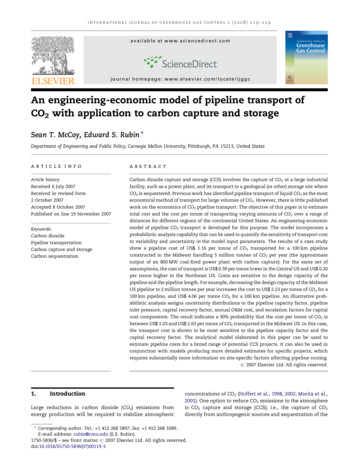
220international journal of greenhouse gas control 2 (2008) 219–229CO2 geological sinks for significant periods of time (Bachu,2003). CCS requires CO2 to be captured from large-scaleindustrial processes, compressed to high pressures, transported to a storage site, and injected into a suitable geologicalformation where it is sequestered and kept from the atmosphere. Studies indicate that under appropriate policyregimes, CCS could act as a potential ‘‘bridging technology’’that would achieve significant CO2 emission reductions whileallowing fossil fuels to be used until alternative energy sourcesare more widely deployed. Moreover, as part of a portfolio ofemissions reducing technologies, CCS could substantiallyreduce the cost of achieving stabilization goals (Herzoget al., 2005).CCS will have significant impacts on the cost of electricityproduction and costs in other potential applications. Thus,methods are required to estimate the costs of CCS to evaluateactions and policies related to the deployment of CCS projects.In the last decade the understanding of CCS technologies hasincreased greatly, as reflected by the recent IPCC SpecialReport on Carbon Dioxide Capture and Storage (Metz et al.,2005). However, there are still significant gaps in knowledge ofthe cost of integrated capture, transport, and storageprocesses. For example, many studies of carbon captureprocesses have been undertaken (Thambimuthu et al., 2005)and engineering-economic models linking process cost to keyengineering parameters have been developed (Rao and Rubin,2002), but the majority have not yet been linked with transportand storage models to determine the cost of an integrated CCSprocess. Most cost studies either exclude transport andstorage costs or assume a constant cost per tonne of CO2 inaddition to capture costs (Metz et al., 2005).There have been few studies that have addressed the costof CO2 transport and storage in detail. However, earlier workby Svensson et al. (2004) identified pipeline transport as themost practical method to move large volumes of CO2 overlandand other studies have affirmed this conclusion (Doctor et al.,2005). Therefore, this paper focuses on the cost of CO2transport via pipeline. Skovholt (1993) presented rules ofthumb for sizing of CO2 pipelines and estimated the capitalcost of pipeline transport. In 2002, the International EnergyAgency Greenhouse Gas Programme (IEA GHG) released areport that presented several correlations for the cost of CO2pipelines in Europe based on detailed case study designs(Woodhill Engineering Consultants, 2002). More recently, anengineering-economic CO2 pipeline model was developed atthe Massachusetts Institute of Technology (MIT) (Bock et al.,2003). Results from these and similar studies were summarized in the recent IPCC report (Doctor et al., 2005). However,none of these studies considered the unusual physicalproperties of CO2 at high pressures (Fesmire, 1983), therealities of available pipeline diameters and costs, or regionaldifferences in the cost of CO2 transportation.The objective of this paper is to estimate the cost per tonneof transporting CO2 for a range of CO2 flow rates (e.g., reflectingdifferent power plant sizes) over a range of distances, and toalso incorporate regional cost differences within the continental US. These cost estimates are embodied in anengineering-economic model that will be presented in thispaper. A probabilistic analysis is used to quantify the impact ofuncertainty and variability in cost model parameters on CO2transport cost. This analysis also shows the range of costsassociated with a given project and the probability of a givencost for a specific scenario.2.Properties of CO2 in pipeline transportEfficient transport of CO2 via pipeline requires that CO2 becompressed and cooled to the liquid state (Zhang et al., 2006).Transport at lower densities (i.e., gaseous CO2) is inefficientbecause of the low density of the CO2 and relatively highpressure drop per unit length. Moreover, by operating thepipeline at pressures greater than the CO2 critical pressure of7.38 MPa, temperature fluctuations along the pipeline will notresult in the formation of gaseous CO2 and the difficultiesencountered with two-phase flow (Recht, 1984).The properties of CO2 are considerably different from otherfluids commonly transported by pipeline, such as natural gas.Thus, it is necessary to use accurate representations of thephase behavior, density, and viscosity of CO2 and CO2containing mixtures in the design of the pipeline. The resultspresented here are based on the physical properties (i.e.,density and phase behavior) of CO2 and CO2-containingmixtures calculated using a cubic equation of state withPeng–Robinson parameters, and mixing rules employing abinary interaction parameter (Reid et al., 1987). The transportproperties of CO2 have been estimated using the Chung et al.(1988) method, extended to high pressures by Reid et al. (1987).Fig. 1 shows that the compressibility of CO2 is non-linear inthe range of pressures common for pipeline transport and ishighly sensitive to any impurities, such as hydrogen sulfide(H2S). Fig. 1 also shows the significant difference between thecompressibility of pure CO2 and CO2 with 10 vol. % H2S. Toreduce difficulties in design and operation, it is generallyrecommended that a CO2 pipeline operate at pressures greaterthan 8.6 MPa where the sharp changes in compressibility ofCO2 can be avoided across a range of temperatures that may beencountered in the pipeline system (Farris, 1983). Conversely,line-pipe with ASME-ANSI 900# flanges has a maximumallowable operating pressure of 15.3 MPa at 38 8C (Mohitpouret al., 2003). Operating the pipeline at higher pressures wouldrequire flanges with a higher rating. Over the range of typicalconditions shown in Fig. 1, the density of CO2 varies betweenapproximately 800 and 1000 kg/m3.Operating temperatures of CO2 pipelines are generallydictated by the temperature of the surrounding soil. Innorthern latitudes, the soil temperature varies from a fewdegrees below zero in the winter to 6–8 8C in summer, while intropical locations; the soil temperature may reach up to 20 8C(Skovholt, 1993). However, at the discharge of compressionstations after-cooling of compressed CO2 may be required toensure that the temperature of CO2 does not exceed theallowable limits for either the pipeline coating or the flangetemperature.3.Pipeline performance modelWhile there are proven flow equations available for use withhigh pressure gas pipelines (e.g., AGA fully turbulent equation),
international journal of greenhouse gas control 2 (2008) 219–229221points 1 and 2, which are upstream and downstream, respectively; h is the pipeline elevation, where 1 and 2 representupstream and downstream locations.Fort the case of a CO2 pipeline modeled here, the averagetemperature, Tave, is assumed to be constant at groundtemperature so that Tave Tground. Because pressurevaries non-linearly along the pipeline, the average pressure,Pave, required in Eq. (2) is calculated (Mohitpour et al.,2003):Pave ¼Fig. 1 – The compressibility of CO2 based on the Peng–Robinson equation of state, showing the nonlinearity inthe typical pipeline transport region and the sensitivity toimpurities, such as 10% H2S (by mole fraction).23 p2 þ p1 p2 p1p2 þ p1 (3)Thus, Eq. (2) can be used to calculate the pipe diameterrequired for a given pressure drop. Complicating this,however, is the Fanning friction factor, which is a functionof the pipe diameter. The Fanning friction factor cannot besolved for analytically; however, an explicit approximation forFanning friction factor is given by Eq. (4) (Zigrang andSylvester, 1982): 1e Di 5:02e Di 5:02e Di 13pffiffiffiffiffiffi ¼ 2:0 logloglog þReRe3:73:73:7 Re2 fF(4)these equations can introduce error into the estimation of flowrates in liquid CO2 due to the underlying assumptions made intheir development (Farris, 1983). The pipeline performancemodel used here is based on an energy balance on the flowingCO2, where the required pipeline diameter for a pipelinesegment is calculated while holding the upstream and downstream pressures constant. The mechanical energy balance canbe written as (Mohitpour et al., 2003):2 f c2c1gdu þ d p þ 2 dh þ F dL ¼ 0vvvDi(1)where c is a constant equal to the product of density, r (kg/m3), and fluid velocity, u (m/s); g is acceleration due to gravity(m/s2); v is the specific volume of fluid (m3/kg); p is pressure(Pa); h is height (m); fF is the fanning friction factor; Di is theinternal pipeline diameter (m); L is the pipeline segmentlength (m).The energy balance given in Eq. (1) can be simplified byassuming that changes in kinetic energy of the flowing CO2 arenegligible (constant velocity), and that the compressibility ofthe CO2 or CO2-containing mixture can be averaged over thelength of the pipeline. The resulting energy balance, as derivedby Mohitpour et al. (2003), and solved for pipe segmentdiameter:(Di ¼)1 5 64Z2ave R2 T2ave f F ṁ2 Lp2 ½MZave RTave ð p22 p21 Þ þ 2gP2ave M2 ðh2 h1 Þ (2)where Zave is the average fluid compressibility; R is the universal gas constant (Pa m3/mol K); Tave is the average fluidtemperature (K); ṁ is the design mass flow rate (kg/s); M isthe molecular weight of the stream (kg/kgmol); p is pressure atwhere e is the roughness of the pipe (m), which is approximately 0.0457 mm for commercial steel pipe (Boyce, 1997), andRe is the Reynolds number, which is defined as (McCabe et al.,1993):Re ¼4ṁmpDi(5)where m is the viscosity of the fluid (Pa s). As a result, Eqs. (2),(4), and (5) must be solved iteratively to determine the pipediameter required for a particular application. In the iteration scheme shown in Fig. 2, the Reynolds number, Eq. (5), isfirst calculated using an initial estimate of pipe diameterbased on a velocity of 1.36 m/s. This initial velocity is representative of CO2 pipeline flows, and thus minimizes thenumber of iterations required over a range of model inputsfor both design mass flow rate and pipeline length. Thecalculated Reynolds number is then used in Eq. (4) to estimate the Fanning friction factor, which is then substitutedinto Eq. (2). This yields an updated diameter, which is compared with the value at the previous iteration. Values for theinternal diameter converge to within 10 6 m in generally lessthan five iterations.Line pipe is not available in continuous diameters. Thusthe internal pipe diameter calculated must be adjusted toaccount for both available pipe diameters and the pipe wallthickness. A discrete size of line pipe is frequently referred toby its Nominal Pipe Size (NPS), which corresponds approximately to the outside pipe diameter measured in inches. Inthe model presented here, eleven NPS values between 4 and30 are available. To determine the inside diameter, the pipewall thickness (also known as the pipe schedule) for each NPSis estimated using the method specified in the US Code ofFederal Regulations (CFR), which regulates the design,construction, and operation of CO2 pipelines in the United
222international journal of greenhouse gas control 2 (2008) 219–229Fig. 2 – Flowchart illustrating the calculation method used to estimate the pipeline diameter.States. The pipe wall thickness, t, in meters is given as (CFR,2005):t¼pmop Do2SEF(6)where pmop is the maximum operating pressure of the pipeline (Pa), Do is the outside pipe diameter (m), S is the specifiedminimum yield stress for the pipe material (Pa), E is thelongitudinal joint factor (reflecting different types of longitudinal pipe welds), and F is the design factor (introduced toadd a margin of safety to the wall thickness calculation). Forthe purposes of estimating the pipe wall thickness, themaximum operating pressure is assumed to be 15.3 MPa,the longitudinal joint factor is 1.0, and the design factor is0.72 (as required in the CFR). The minimum yield stress isdependent on the specification and grade of line pipeselected for the pipeline. For CO2 service, pipelines are generally constructed with materials meeting American Petroleum Institute (API) specification 5L (American PetroleumInstitute, 2004). In this case, the minimum yield stress hasbeen specified as 483 MPa, which corresponds to API 5L X-70line pipe.The value of Di calculated from Eq. (2) is adjusted to the nextlarges value of Di for an available NPS. Based on the adjustedDi, the adjusted downstream pressure for the pipelinesegment is calculated. This pressure will always be greaterthan the downstream pressure specified by the user since theadjusted diameter will always be greater than the optimumvalue calculated by Eq. (2).Fig. 3 shows the NPS of a pipeline carrying pure CO2 asa function of the design CO2 mass flow rate, as calculatedby the iteration scheme shown in Fig. 2. For fixed inletpressure and minimum outlet pressure, the required pipediameter increases with increasing design CO2 flow rateand pipeline distance. Steps in pipeline diameter occurbecause of the discrete NPS available in the model. Forexample, the model estimates an internal diameterof 0.38 m for a pipeline spanning a distance of 100 kmdesigned to carry 5 million tonnes per year of CO2 ata pressure drop of 35 kPa/km. However, this is not acommon line pipe size; thus, the next largest NPS is selected
international journal of greenhouse gas control 2 (2008) 219–229223Fig. 4 – The six US regions used in the pipeline transportcost model.Fig. 3 – Required pipe diameter for the specified inlet andoutlet pressures, for different pipeline lengths and fourdifferent design mass flow rates, as predicted by theperformance model.by the model, which has an internal diameter of about0.39 m.4.Pipeline cost modelDetailed construction cost data for actual CO2 pipelines (i.e.,as-built-cost including the length and diameter) are notreadily available; nor have many such projects been constructed in the last decade (Doctor et al., 2005). For thesereasons, the data set used to develop the pipeline capital costmodels is based on natural gas pipelines. However, there aremany similarities between transport of natural gas and CO2.Both are transported at similar pressures, approximately10 MPa and greater. Assuming the CO2 is dry, which is acommon requirement for CCS, both pipelines will requiresimilar materials. Thus, a model based on natural gaspipelines offers a reasonable approximation for a preliminarydesign model used in the absence of more detailed projectspecific costs.The CO2 pipeline capital cost model is based on regressionanalyses of natural gas pipeline project costs publishedbetween 1995 and 2005 (True, 1995, 1996, 1997, 1999,2000a,b, 2001, 2002, 2003a,b; True and Stell, 2004; Smithet al., 2005). These project costs are based on Federal EnergyRegulatory Commission (FERC) filings from interstate gastransmission companies. The entire data set contains the ‘‘asbuilt’’ costs for 263 on-shore pipeline projects in thecontiguous 48-states and excludes costs for pipelines withriver or stream crossings as well as lateral pipeline projects(i.e., a pipeline of secondary significance to the mainlinesystem, such as a tie-in between the mainline and a powerplant). Costs from each year’s projects have been adjusted to2004 dollars using the Marshall and Swift equipment costindex (Chemical Engineering, 2006).The pipeline data set contains information on the yearand location of the project and the length and diameterof the pipeline. Locations are listed by state in the dataset; however, to develop the regression models presentedhere, the states have been grouped into six geographicalregions. The project regions used here are the same asthose used by the Energy Information Administration(2006) for natural gas pipeline regions, and are shown inFig. 4.The total construction cost for each project is broken downinto four categories: materials, labor, right-of-way (ROW), andmiscellaneous charges. The materials category includes thecost of line pipe, pipe coatings, and cathodic protection. Laboris the cost of pipeline construction labor. ROW covers the costof obtaining right-of-way for the pipeline and allowance fordamages to landowners’ property during construction. Miscellaneous includes the costs of surveying, engineering,supervision, contingencies, telecommunications equipment,freight, taxes, allowances for funds used during construction(AFUDC), administration and overheads, and regulatory filingfees.Separate cost models have been developed for each of thecost categories. The capital cost models take this generalform:logðCÞ ¼ a0 þ a1 NE þ a2 SE þ a3 CL þ a4 SW þ a5 Wþ a6 logðLÞ þ a7 logðDnps Þ(7)where NE, SE, CL, SW, and W are binary variables reflecting thefive geographic regions besides Midwest (i.e., Northeast,Southeast, Central, Southwest, and West, respectively) thattake a value of 1 or 0 depending on the region and increase ordecrease the estimated cost relative to the Midwest value. C isthe pipeline capital cost in 2004 US dollars. The variable L is thetotal pipeline length in kilometers, and the D is the pipelineNPS. Regional variables exist in the cost model only if they arestatistically significant predictors of the cost; thus differentcost-component models include different sets of regionalvariables.
224international journal of greenhouse gas control 2 (2008) 219–229Table 1 – Regression coefficients for the pipeline cost model, Eq. (7); with standard errors indicated in parenthesesCoefficient estimateCost .045)LaborROW****4.487 (0.109)0.075* (0.032)– 0.187** (0.048) 0.216** (0.059)–0.820** (0.023)0.940** (0.077)3.950 (0.244)–– 0.382** (0.093)––1.049** (0.048)0.403* (0.167)Miscellaneous4.390** (0.132)0.145** (0.045)0.132* (0.054) 0.369** (0.061)– 0.377** (0.066)0.783** (0.027)0.791** (0.091)Significant at the 5% level.Significant at the 1% level.If the intercept and regional variables in Eq. (7) are collectedinto a single term and rearranged, the cost model can berewritten in Cobb-Douglas form1:7;C ¼ bLa6 Danps(8)where logðbÞ ¼ a0 þ a1 NE þ a2 SE þ a3 CL þ a4 SW þ a5 WThere are several properties of Cobb-Douglas functions thatare of interest in the context of the cost models. If the sum of a6and a7 is equal to one, the capital cost exhibits constantreturns to scale (i.e., cost is linear with L and D). If the sumis less than one, there are decreasing returns to scale, and ifthe sum is greater than one, increasing returns to scale. Moreover, the values of a6 and a7 represent the elasticity of costwith respect to length and diameter, respectively.Parameter estimates for the materials, labor, miscellaneous charges, and ROW cost components are given inTable 1. The generalized regression model given in Eq. (7)accounts for a large proportion of the variation in the dataset for each of the cost categories, as reflected by all of thecost component models having an adjusted-r2 value greaterthan 0.81, with the exception of ROW, which has anadjusted-r2 value of 0.67.Based on the regression results shown in Table 1, severalgeneral observations can be made. The cost of all fourcomponents exhibit increasing returns to scale, whichmeans that multiplying both the length and diameter by aconstant n multiplies the materials cost by a factor greaterthan n. For example, doubling both pipeline length anddiameter results in a nearly 6-fold (rather than 4-fold)increase in materials cost. For the materials, labor andmiscellaneous costs, the elasticity of substitution for lengthis less than one; thus, a doubling in pipeline length results inless than a doubling of the cost for these components (oftenreferred to as economies of scale). However, the elasticity ofsubstitution for length in the ROW cost is approximatelyone, so that doubling the length results in a doubling of ROWcost (which is reasonable, as the ROW cost per unit of landshould be approximately constant regardless of the pipelinelength). The elasticity of substitution for pipeline diameter is1In economic theory, a Cobb-Douglas production function hasthe form f(K,L) AKaLb, where K and L traditionally refer to capitaland labor.less than one for labor, miscellaneous, and ROW costs, againindicating economies of scale; however, for materials cost itis approximately 1.6, so that doubling the pipeline diameterresults in a 3-fold materials cost increase. Note that this stillreflects an economy of scale in the total cost of materialssince doubling the diameter would quadruple the total massof steel needed.At least one regional variable was found to be statisticallysignificant in all of the regression model cost categories,implying that for some regions, the cost of constructing apipeline is higher or lower than the average for the Midwestregion. For example, the labor cost regression results (Table 1)show that the cost multiplier is approximately US 6000greater in the Northeast than the Midwest and approximatelyUS 10,000 lower in the Central and Southwest regions. Thereis no statistical difference (at the 5% level) between theMidwest and West or Southeast cost intercepts.Cost differences between regions could be caused by acombination of two types of factors: differences betweenregions in the average cost of materials, labor, miscellaneouscosts, and land (affecting ROW cost); and, differences inother geographic factors, such as population density andterrain. Regional variation in labor and materials cost forpower plant construction have been documented by theElectric Power Research Institute (EPRI) (Electric PowerResearch Institute, 1993). However, because the routings ofpipeline projects are not reported in the data set, it is notpossible to identify how these individual factors contributedto overall cost of the projects. Thus, there are plausiblecircumstances where similar pipeline projects in differentregions could have costs much closer to one another than tocomparable projects within their respective regions (e.g.,pipelines of similar length and design CO2 mass flow inheavily populated versus unpopulated areas within thesame state). Zhang et al. (2007) have developed more dataintensive tools to study least-cost routing of specific CO2pipelines which are complimentary to the use of the currentscreening level model.While operating and maintenance (O&M) costs are notlarge in comparison to the annualized capital cost of pipelinetransport, they are nonetheless significant. Bock et al. (2003)report that the O&M cost of operating a 480 km CO2 pipeline isbetween US 40,000 and US 60,000 per month. On an annualbasis, this amounts to approximately US 3250 per kilometerof pipeline in 2004 dollars.
225international journal of greenhouse gas control 2 (2008) 219–229Table 2 – Illustrative case study values for the model parametersModel parameterDeterministic valuePipeline parametersDesign mass flow (Mt/year)Pipeline length (km)Pipeline capacity factor (%)Ground temperature (8C)Inlet pressure (MPa)Minimum outlet pressure (MPa)Pipe roughness (mm)51001001213.7910.30.0457Economic and financial parametersProject regionCapital recovery factor (%)Annual O&M cost (US /km/year)Escalation factor for materials costEscalation factor for labor costEscalation factor for ROW costEscalation factor for miscellaneous costMidwest15b32501111abUncertainty distributionVariableaVariableaUniform (50, 100)Uniform (12, 15)UniformUniformUniformUniformUniformUniform(10, 20)(2150, 4350)(0.75, 1.25)(0.75, 1.25)(0.75, 1.25)(0.75, 1.25)This parameter is modeled as a series of discrete values.Corresponds to a 30-year plant lifetime with a 14.8% real interest rate (or, a 20-year life with 13.9% interest rate).5.Combining performance and costTo facilitate calculations, the linked pipeline performance andcost models have been programmed as a stand-alone spreadsheet model using Visual Basic in Microsoft Excel. Implementation of all equations has been validated by comparingspreadsheet results to manually calculated results using thesame input parameters. The pipeline model has also beenimplemented in the Integrated Environmental Control Model(IECM), a power plant simulation model developed by CarnegieMellon University for the U.S. Department of Energy (USDOE) toestimate the performance, emissions, and cost of alternativepower generation technologies and emissions control options(Rao and Rubin, 2002; Berkenpas et al., 2004). The new CO2pipeline transport module allows the IECM to analyze in greaterdetail the performance and cost of alternative CO2 capture andsequestration technologies in complex plant designs involvingmultipollutant emission controls.The key results reported by the newly developed pipelinemodel include the total capital cost, annual O&M cost, totallevelized cost, and the levelized cost per metric tonnes of CO2transported (all in constant 2004 US dollars). The capital costcan be subject to capital cost escalation factors applied toindividual categories of the capital cost (i.e., materials, labor,miscellaneous, and ROW). These escalation factors can beused to account for anticipated changes in capital costcomponents (e.g., in the cost of steel) or other project-specificfactors that might affect capital costs relative to the regionalaverages discussed earlier (e.g., river crossings). Capital costsare annualized using a levelized fixed charge factor calculatedfor a user-specified discount rate and project life (Berkenpaset al., 2004). The cost per tonne CO2 transported reflects theamount of CO2 transported, which is the product of the designmass flow rate and the pipeline capacity factor.6.Case study resultsIllustrative results from the pipeline model were developedusing parameters representative of a typical coal-fired powerplant in the Midwest region of the United States (Table 2).Several parameter values (e.g., capital recovery factor) aredefault values from the IECM software. Table 2 includes anominal CO2 mass flow rate and pipeline length, but these twoparameters are varied parametrically in the case study resultspresented here.Table 3 – The levelized cost of pipeline transport in the Midwest and regional differences relative to the Midwest, based onassumptions in Table 2Transport cost (US /tonne CO2)MidwestDifference from midwest costNortheastSoutheastSou
by Svensson et al. (2004) identified pipeline transport as the mostpractical methodto move largevolumesof CO 2 overland and other studies have affirmed this conclusion (Doctor et al., 2005). Therefore, this paper focuses on the cost of CO 2 transport via pipeline. Skovholt (1993) presented rul