Transcription
Linear Algebra in Twenty Five LecturesTom Denton and Andrew WaldronMarch 27, 2012Edited by Katrina Glaeser, Rohit Thomas & Travis Scrimshaw1
Contents1 What is Linear Algebra?122 Gaussian Elimination192.1 Notation for Linear Systems . . . . . . . . . . . . . . . . . . . 192.2 Reduced Row Echelon Form . . . . . . . . . . . . . . . . . . . 213 Elementary Row Operations274 Solution Sets for Systems of Linear Equations344.1 Non-Leading Variables . . . . . . . . . . . . . . . . . . . . . . 355 Vectors in Space, n-Vectors435.1 Directions and Magnitudes . . . . . . . . . . . . . . . . . . . . 466 Vector Spaces537 Linear Transformations588 Matrices639 Properties of Matrices729.1 Block Matrices . . . . . . . . . . . . . . . . . . . . . . . . . . 729.2 The Algebra of Square Matrices . . . . . . . . . . . . . . . . 7310 Inverse Matrix10.1 Three Properties of the Inverse10.2 Finding Inverses . . . . . . . . .10.3 Linear Systems and Inverses . .10.4 Homogeneous Systems . . . . .10.5 Bit Matrices . . . . . . . . . . .79808182838411 LU Decomposition8811.1 Using LU Decomposition to Solve Linear Systems . . . . . . . 8911.2 Finding an LU Decomposition. . . . . . . . . . . . . . . . . . 9011.3 Block LDU Decomposition . . . . . . . . . . . . . . . . . . . . 942
12 Elementary Matrices and Determinants9612.1 Permutations . . . . . . . . . . . . . . . . . . . . . . . . . . . 9712.2 Elementary Matrices . . . . . . . . . . . . . . . . . . . . . . . 10013 Elementary Matrices and Determinants II10714 Properties of the Determinant11614.1 Determinant of the Inverse . . . . . . . . . . . . . . . . . . . . 11914.2 Adjoint of a Matrix . . . . . . . . . . . . . . . . . . . . . . . . 12014.3 Application: Volume of a Parallelepiped . . . . . . . . . . . . 12215 Subspaces and Spanning Sets12415.1 Subspaces . . . . . . . . . . . . . . . . . . . . . . . . . . . . . 12415.2 Building Subspaces . . . . . . . . . . . . . . . . . . . . . . . . 12616 Linear Independence13117 Basis and Dimension139n17.1 Bases in R . . . . . . . . . . . . . . . . . . . . . . . . . . . . . 14218 Eigenvalues and Eigenvectors14718.1 Matrix of a Linear Transformation . . . . . . . . . . . . . . . 14718.2 Invariant Directions . . . . . . . . . . . . . . . . . . . . . . . . 15119 Eigenvalues and Eigenvectors II15919.1 Eigenspaces . . . . . . . . . . . . . . . . . . . . . . . . . . . . 16220 Diagonalization16520.1 Diagonalization . . . . . . . . . . . . . . . . . . . . . . . . . . 16520.2 Change of Basis . . . . . . . . . . . . . . . . . . . . . . . . . . 16621 Orthonormal Bases17321.1 Relating Orthonormal Bases . . . . . . . . . . . . . . . . . . . 17622 Gram-Schmidt and Orthogonal Complements18122.1 Orthogonal Complements . . . . . . . . . . . . . . . . . . . . 18523 Diagonalizing Symmetric Matrices3191
24 Kernel, Range, Nullity, Rank19724.1 Summary . . . . . . . . . . . . . . . . . . . . . . . . . . . . . 20125 Least Squares206A Sample Midterm I Problems and Solutions211B Sample Midterm II Problems and Solutions221C Sample Final Problems and Solutions231D Points Vs. Vectors256E Abstract ConceptsE.1 Dual Spaces . .E.2 Groups . . . . .E.3 Fields . . . . .E.4 Rings . . . . . .E.5 Algebras . . . .F Sine and Cosine as an Orthonormal BasisG Movie ScriptsG.1 Introductory Video . . . . . . . . . . . . . . . . . . . . . . .G.2 What is Linear Algebra: Overview . . . . . . . . . . . . . .G.3 What is Linear Algebra: 3 3 Matrix Example . . . . . . .G.4 What is Linear Algebra: Hint . . . . . . . . . . . . . . . . .G.5 Gaussian Elimination: Augmented Matrix Notation . . . . .G.6 Gaussian Elimination: Equivalence of Augmented Matrices .G.7 Gaussian Elimination: Hints for Review Questions 4 and 5 .G.8 Gaussian Elimination: 3 3 Example . . . . . . . . . . . . .G.9 Elementary Row Operations: Example . . . . . . . . . . . .G.10 Elementary Row Operations: Worked Examples . . . . . . .G.11 Elementary Row Operations: Explanation of Proof for Theorem 3.1 . . . . . . . . . . . . . . . . . . . . . . . . . . . . . .G.12 Elementary Row Operations: Hint for Review Question 3 .G.13 Solution Sets for Systems of Linear Equations: Planes . . . .G.14 Solution Sets for Systems of Linear Equations: Pictures andExplanation . . . . . . . . . . . . . . . . . . . . . . . . . . .4.258258258259260261262264. 264. 265. 267. 268. 269. 270. 271. 273. 274. 277. 279. 281. 282. 283
G.15 Solution Sets for Systems of Linear Equations: Example . . . 285G.16 Solution Sets for Systems of Linear Equations: Hint . . . . . . 287G.17 Vectors in Space, n-Vectors: Overview . . . . . . . . . . . . . 288G.18 Vectors in Space, n-Vectors: Review of Parametric Notation . 289G.19 Vectors in Space, n-Vectors: The Story of Your Life . . . . . . 291G.20 Vector Spaces: Examples of Each Rule . . . . . . . . . . . . . 292G.21 Vector Spaces: Example of a Vector Space . . . . . . . . . . . 296G.22 Vector Spaces: Hint . . . . . . . . . . . . . . . . . . . . . . . . 297G.23 Linear Transformations: A Linear and A Non-Linear Example 298G.24 Linear Transformations: Derivative and Integral of (Real) Polynomials of Degree at Most 3 . . . . . . . . . . . . . . . . . . . 300G.25 Linear Transformations: Linear Transformations Hint . . . . . 302G.26 Matrices: Adjacency Matrix Example . . . . . . . . . . . . . . 304G.27 Matrices: Do Matrices Commute? . . . . . . . . . . . . . . . . 306G.28 Matrices: Hint for Review Question 4 . . . . . . . . . . . . . . 307G.29 Matrices: Hint for Review Question 5 . . . . . . . . . . . . . . 308G.30 Properties of Matrices: Matrix Exponential Example . . . . . 309G.31 Properties of Matrices: Explanation of the Proof . . . . . . . . 310G.32 Properties of Matrices: A Closer Look at the Trace Function . 312G.33 Properties of Matrices: Matrix Exponent Hint . . . . . . . . . 313G.34 Inverse Matrix: A 2 2 Example . . . . . . . . . . . . . . . . 315G.35 Inverse Matrix: Hints for Problem 3 . . . . . . . . . . . . . . . 316G.36 Inverse Matrix: Left and Right Inverses . . . . . . . . . . . . . 317G.37 LU Decomposition: Example: How to Use LU Decomposition 319G.38 LU Decomposition: Worked Example . . . . . . . . . . . . . . 321G.39 LU Decomposition: Block LDU Explanation . . . . . . . . . . 322G.40 Elementary Matrices and Determinants: Permutations . . . . 323G.41 Elementary Matrices and Determinants: Some Ideas Explained 324G.42 Elementary Matrices and Determinants: Hints for Problem 4 . 327G.43 Elementary Matrices and Determinants II: Elementary Determinants . . . . . . . . . . . . . . . . . . . . . . . . . . . . . . 328G.44 Elementary Matrices and Determinants II: Determinants andInverses . . . . . . . . . . . . . . . . . . . . . . . . . . . . . . 330G.45 Elementary Matrices and Determinants II: Product of Determinants . . . . . . . . . . . . . . . . . . . . . . . . . . . . . . 332G.46 Properties of the Determinant: Practice taking Determinants 333G.47 Properties of the Determinant: The Adjoint Matrix . . . . . . 335G.48 Properties of the Determinant: Hint for Problem 3 . . . . . . 3385
G.49 Subspaces and Spanning Sets: Worked Example . . . . . . .G.50 Subspaces and Spanning Sets: Hint for Problem 2 . . . . . .G.51 Subspaces and Spanning Sets: Hint . . . . . . . . . . . . . .G.52 Linear Independence: Worked Example . . . . . . . . . . . .G.53 Linear Independence: Proof of Theorem 16.1 . . . . . . . . .G.54 Linear Independence: Hint for Problem 1 . . . . . . . . . . .G.55 Basis and Dimension: Proof of Theorem . . . . . . . . . . .G.56 Basis and Dimension: Worked Example . . . . . . . . . . . .G.57 Basis and Dimension: Hint for Problem 2 . . . . . . . . . . .G.58 Eigenvalues and Eigenvectors: Worked Example . . . . . . .G.59 Eigenvalues and Eigenvectors: 2 2 Example . . . . . . . .G.60 Eigenvalues and Eigenvectors: Jordan Cells . . . . . . . . . .G.61 Eigenvalues and Eigenvectors II: Eigenvalues . . . . . . . . .G.62 Eigenvalues and Eigenvectors II: Eigenspaces . . . . . . . . .G.63 Eigenvalues and Eigenvectors II: Hint . . . . . . . . . . . . .G.64 Diagonalization: Derivative Is Not Diagonalizable . . . . . .G.65 Diagonalization: Change of Basis Example . . . . . . . . . .G.66 Diagonalization: Diagionalizing Example . . . . . . . . . . .G.67 Orthonormal Bases: Sine and Cosine Form All OrthonormalBases for R2 . . . . . . . . . . . . . . . . . . . . . . . . . . .G.68 Orthonormal Bases: Hint for Question 2, Lecture 21 . . . . .G.69 Orthonormal Bases: Hint . . . . . . . . . . . . . . . . . . .G.70 Gram-Schmidt and Orthogonal Complements: 4 4 GramSchmidt Example . . . . . . . . . . . . . . . . . . . . . . . .G.71 Gram-Schmidt and Orthogonal Complements: Overview . .G.72 Gram-Schmidt and Orthogonal Complements: QR Decomposition Example . . . . . . . . . . . . . . . . . . . . . . . . .G.73 Gram-Schmidt and Orthogonal Complements: Hint for Problem 1 . . . . . . . . . . . . . . . . . . . . . . . . . . . . . . .G.74 Diagonalizing Symmetric Matrices: 3 3 Example . . . . . .G.75 Diagonalizing Symmetric Matrices: Hints for Problem 1 . . .G.76 Kernel, Range, Nullity, Rank: Invertibility Conditions . . . .G.77 Kernel, Range, Nullity, Rank: Hint for 1 . . . . . . . . . .G.78 Least Squares: Hint for Problem 1 . . . . . . . . . . . . . .G.79 Least Squares: Hint for Problem 2 . . . . . . . . . . . . . .H Student 358360361362363368. 370. 371. 372. 374. 376. 378.3803823843853863873883896
IOther Resources390J List of Symbols392Index3937
PrefaceThese linear algebra lecture notes are designed to be presented as twenty five,fifty minute lectures suitable for sophomores likely to use the material forapplications but still requiring a solid foundation in this fundamental branchof mathematics. The main idea of the course is to emphasize the conceptsof vector spaces and linear transformations as mathematical structures thatcan be used to model the world around us. Once “persuaded” of this truth,students learn explicit skills such as Gaussian elimination and diagonalizationin order that vectors and linear transformations become calculational tools,rather than abstract mathematics.In practical terms, the course aims to produce students who can performcomputations with large linear systems while at the same time understandthe concepts behind these techniques. Often-times when a problem can be reduced to one of linear algebra it is “solved”. These notes do not devote muchspace to applications (there are already a plethora of textbooks with titlesinvolving some permutation of the words “linear”, “algebra” and “applications”). Instead, they attempt to explain the fundamental concepts carefullyenough that students will realize for their own selves when the particularapplication they encounter in future studies is ripe for a solution via linearalgebra.There are relatively few worked examples or illustrations in these notes,this material is instead covered by a series of “linear algebra how-to videos”. The “scripts”They can be viewed by clicking on the take one iconfor these movies are found at the end of the notes if students prefer to readthis material in a traditional format and can be easily reached via the scripticon. Watch an introductory video below:Introductory VideoThe notes are designed to be used in conjunction with a set of onlinehomework exercises which help the students read the lecture notes and learnbasic linear algebra skills. Interspersed among the lecture notes are linksto simple online problems that test whether students are actively readingthe notes. In addition there are two sets of sample midterm problems withsolutions as well as a sample final exam. There are also a set of ten online assignments which are usually collected weekly. The first assignment8
is designed to ensure familiarity with some basic mathematic notions (sets,functions, logical quantifiers and basic methods of proof). The remainingnine assignments are devoted to the usual matrix and vector gymnasticsexpected from any sophomore linear algebra class. These exercises are allavailable WaldronWinter-2012/Webwork is an open source, online homework system which originated atthe University of Rochester. It can efficiently check whether a student hasanswered an explicit, typically computation-based, problem correctly. Theproblem sets chosen to accompany these notes could contribute roughly 20%of a student’s grade, and ensure that basic computational skills are mastered.Most students rapidly realize that it is best to print out the Webwork assignments and solve them on paper before entering the answers online. Thosewho do not tend to fare poorly on midterm examinations. We have foundthat there tend to be relatively few questions from students in office hoursabout the Webwork assignments. Instead, by assigning 20% of the gradeto written assignments drawn from problems chosen randomly from the review exercises at the end of each lecture, the student’s focus was primarilyon understanding ideas. They range from simple tests of understanding ofthe material in the lectures to more difficult problems, all of them requirethinking, rather than blind application of mathematical “recipes”. Officehour questions reflected this and offered an excellent chance to give studentstips how to present written answers in a way that would convince the persongrading their work that they deserved full credit!Each lecture concludes with references to the comprehensive online textbooks of Jim Hefferon and Rob //linear.ups.edu/index.htmland the notes are also hyperlinked to Wikipedia where students can rapidlyaccess further details and background material for many of the concepts.Videos of linear algebra lectures are available online from at least two sources: The Khan Academy,http://www.khanacademy.org/?video#Linear Algebra9
MIT OpenCourseWare, Professor Gilbert 6-linear-algebra-spring-2010/video-lectures/There are also an array of useful commercially available texts.exhaustive list includesA non- “Introductory Linear Algebra, An Applied First Course”, B. Kolmanand D. Hill, Pearson 2001. “Linear Algebra and Its Applications”, David C. Lay, Addison–Weseley2011. “Introduction to Linear Algebra”, Gilbert Strang, Wellesley CambridgePress 2009. “Linear Algebra Done Right”, S. Axler, Springer 1997. “Algebra and Geometry”, D. Holten and J. Lloyd, CBRC, 1978. “Schaum’s Outline of Linear Algebra”, S. Lipschutz and M. Lipson,McGraw-Hill 2008.A good strategy is to find your favorite among these in the University Library.There are many, many useful online math resources. A partial list is givenin Appendix I.Students have also started contributing to these notes. Click here to seesome of their work.There are many “cartoon” type images for the important theorems andformalæ . In a classroom with a projector, a useful technique for instructors isto project these using a computer. They provide a colorful relief for studentsfrom (often illegible) scribbles on a blackboard. These can be downloadedat:Lecture MaterialsThere are still many errors in the notes, as well as awkwardly explainedconcepts. An army of 400 students, Fu Liu, Stephen Pon and Gerry Pucketthave already found many of them. Rohit Thomas has spent a great deal oftime editing these notes and the accompanying webworks and has improvedthem immeasurably. Katrina Glaeser and Travis Scrimshaw have spent many10
hours shooting and scripting the how-to videos and taken these notes to awhole new level! Anne Schilling shot a great guest video. We also thankCaptain Conundrum for providing us his solutions to the sample midtermand final questions. The review exercises would provide a better survey ofwhat linear algebra really is if there were more “applied” questions. Wewelcome your contributions!Andrew and Tom. 2009 by the authors. These lecture notes may be reproduced in theirentirety for non-commercial purposes.11
1What is Linear Algebra?Video OverviewThree bears go into a cave, two come out. Would you go in?Brian ButterworthNumbers are highly useful tools for surviving in the modern world, so muchso that we often introduce abstract pronumerals to represent them:n bears go into a cave, n 1 come out. Would you go in?A single number alone is not sufficient to model more complicated realworld situations. For example, suppose I asked everybody in this room torate the likeability of everybody else on a scale from 1 to 10. In a room fullof n people (or bears sic) there would be n2 ratings to keep track of (howmuch Jill likes Jill, how much does Jill like Andrew, how much does Andrewlike Jill, how much does Andrew like Andrew, etcetera). We could arrangethese in a square array 9 4 ··· 10 6 .Would it make sense to replace such an array by an abstract symbol M ? Inthe case of numbers, the pronumeral n was more than a placeholder for aparticular piece of information; there exists a myriad of mathematical operations (addition, subtraction, multiplication,.) that can be performed withthe symbol n that could provide useful information about the real world system at hand. The array M is often called a matrix and is an example of a12
more general abstract structure called a linear transformation on which manymathematical operations can also be defined. (To understand why having anabstract theory of linear transformations might be incredibly useful and evenlucrative, try replacing “likeability ratings” with the number of times internet websites link to one another!) In this course, we’ll learn about three maintopics: Linear Systems, Vector Spaces, and Linear Transformations. Alongthe way we’ll learn about matrices and how to manipulate them.For now, we’ll illustrate some of the basic ideas of the course in the case oftwo by two matrices. Everything will carefully defined later, we just want tostart with some simple examples to get an idea of the things we’ll be workingwith.Example Suppose I have a bunch of apples and oranges. Let x be the number ofapples I have, and y be the number of oranges I have. As everyone knows, apples andoranges don’t mix, so if I want to keep track of the number of apples and oranges Ihave, I should put them in a list. We’ll call this list a vector, and write it like this:(x, y). The order here matters! I should remember to always write the number ofapples first and then the number of oranges - otherwise if I see the vector (1, 2), Iwon’t know whether I have two apples or two oranges.This vector in the example is just a list of two numbers, so if we wantto, we can represent it with a point in the plane with the correspondingcoordinates, like so:13
Oranges(x, y)ApplesIn the plane, we can imagine each point as some combination of apples andoranges (or parts thereof, for the points that don’t have integer coordinates).Then each point corresponds to some vector. The collection of all suchvectors—all the points in our apple-orange plane—is an example of a vectorspace.Example There are 27 pieces of fruit in a barrel, and twice as many oranges as apples.How many apples and oranges are in the barrel?How to solve this conundrum? We can re-write the question mathematically asfollows:x y 27y 2xThis is an example of a Linear System. It’s a collection of equations inwhich variables are multiplied by constants and summed, and no variablesare multiplied together: There are no powers of x or y greater than one, nofractional or negative powers of x or y, and no places where x and y aremultiplied together.Reading homework: problem 1.1Notice that we can solve the system by manipulating the equations involved. First, notice that the second equation is the same as 2x y 0.Then if you subtract the second equation from the first, you get on the leftside x y ( 2x y) 3x, and on the left side you get 27 0 27. Then14
3x 27, so we learn that x 9. Using the second equation, we then seethat y 18. Then there are 9 apples and 18 oranges.Let’s do it again, by working with the list of equations as an object initself. First we rewrite the equations tidily:x y 272x y 0We can express this set of equations with a matrix as follows: 1 1x27 2 1y0The square list of numbers is an example of a matrix. We can multiplythe matrix by the vector to get back the linear system using the followingrule for multiplying matrices by vectors: a bxax by (1)c dycx dyReading homework: problem 1.2A 3 3 matrix exampleThe matrix is an example of a Linear Transformation, because it takesone vector and turns it into another in a “linear” way.Our next task is to solve linear systems. We’ll learn a general methodcalled Gaussian Elimination.ReferencesHefferon, Chapter One, Section 1Beezer, Chapter SLE, Sections WILA and SSLEWikipedia, Systems of Linear Equations15
Review Problems1. Let M be aM ca matrix and u and v vectors: bxw,v ,u .dyz(a) Propose a definition for u v.(b) Check that your definition obeys M v M u M (u v).2. Matrix Multiplication: Let M and N be matrices a be fM and N ,c dg hand v a vector xv .yCompute the vector N v using the rule given above. Now multiply thisvector by the matrix M , i.e., compute the vector M (N v).Next recall that multiplication of ordinary numbers is associative, namelythe order of brackets does not matter: (xy)z x(yz). Let us try todemand the same property for matrices and vectors, that isM (N v) (M N )v .We need to be careful reading this equation because N v is a vector andso is M (N v). Therefore the right hand side, (M N )v should also be avector. This means that M N must be a matrix; in fact it is the matrixobtained by multiplying the matrices M and N . Use your result forM (N v) to find the matrix M N .3. Pablo is a nutritionist who knows that oranges always have twice asmuch sugar as apples. When considering the sugar intake of schoolchildren eating a barrel of fruit, he represents the barrel like so:16
fruit(s, f )sugarFind a linear transformation relating Pablo’s representation to the onein the lecture. Write your answer as a matrix.Hint: Let λ represent the amount of sugar in each apple.Hint4. There are methods for solving linear systems other than Gauss’ method.One often taught in high school is to solve one of the equations for avariable, then substitute the resulting expression into other equations.That step is repeated until there is an equation with only one variable. From that, the first number in the solution is derived, and thenback-substitution can be done. This method takes longer than Gauss’method, since it involves more arithmetic operations, and is also morelikely to lead to errors. To illustrate how it can lead to wrong conclusions, we will use the systemx 3y 12x y 32x 2y 0(a) Solve the first equation for x and substitute that expression intothe second equation. Find the resulting y.(b) Again solve the first equation for x, but this time substitute thatexpression into the third equation. Find this y.17
What extra step must a user of this method take to avoid erroneouslyconcluding a system has a solution?18
22.1Gaussian EliminationNotation for Linear SystemsIn Lecture 1 we studied the linear systemx y 272x y 0and found thatx 9y 18We learned to write the linear system using a matrix and two vectors like so: 1 1x27 2 1y0Likewise, we can write the solution as: 1 0x9 0 1y18 1 0The matrix I is called the Identity Matrix . You can check that if0 1v is any vector, then Iv v.A useful shorthand for a linear system is an Augmented Matrix , whichlooks like this for the linear system we’ve been dealing with: 1 1 272 1 0 xWe don’t bother writing the vector, since it will show up in anyylinear system we deal with. The solution to the linear system looks like this: 1 0 90 1 1819
Augmented Matrix NotationHere’s another example of an augmented matrix, for a linear system withthree equations and four unknowns: 1 3 2 0 9 6 2 0 2 0 1 0 1 1 3And finally, here’s the general case. The number of equations in the linearsystem is the number of rows r in the augmented matrix, and the number ofcolumns k in the matrix left of the vertical line is the number of unknowns. a11 a12 · · · a1k b1 a2 a2 · · · a2 b 2 k 1 2 . . . . . . ar1 ar2 · · · ark brReading homework: problem 2.1Here’s the idea: Gaussian Elimination is a set of rules for taking a general augmented matrix and turning it into a very simple augmented matrixconsisting of the identity matrix on the left and a bunch of numbers (thesolution) on the right.Equivalence Relations for Linear SystemsEquivalence ExampleIt often happens that two mathematical objects will appear to be different but in fact are exactly the same. The best-known example of this are6fractions. For example, the fractions 12 and 12describe the same number.We could certainly call the two fractions equivalent.In our running example, we’ve noticed that the two augmented matrices20
1 1 27,2 1 0 1 0 90 1 18both contain the same information: x 9, yTwo augmented matrices correspondinghave solutions are said to be (row) equivalentTo denote this, we write: 11 1 27 2 1 00 18.to linear systems that actuallyif they have the same solutions. 0 91 18The symbol is read “is equivalent to”.A small excursion into the philosophy of mathematical notation: SupposeI have a large pile of equivalent fractions, such as 24 , 27, 100 , and so on. Most54 200people will agree that their favorite way to write the number represented byall these different factors is 21 , in which the numerator and denominator arerelatively prime. We usually call this a reduced fraction. This is an exampleof a canonical form, which is an extremely impressive way of saying “favoriteway of writing it down”. There’s a theorem telling us that every rationalnumber can be specified by a unique fraction whose numerator and denominator are relatively prime. To say that again, but slower, every rationalnumber has a reduced fraction, and furthermore, that reduced fraction isunique.A 3 3 example2.2Reduced Row Echelon FormSince there are many different augmented matrices that have the same setof solutions, we should find a canonical form for writing our augmentedmatrices. This canonical form is called Reduced Row Echelon Form, or RREFfor short. RREF looks like this in general:21
1 0 0 ··· 01 0 ··· 001 ··· . . . 00 ··· 0 . .000 ··· 0 b10 b2 0 b3 . 0 . 1 bk 0 0 . . . . 0 0The first non-zero entry in each row is called the pivot. The asterisksdenote arbitrary content which could be several columns long. The followingproperties describe the RREF.1. In RREF, the pivot of any row is always 1.2. The pivot of any given row is always to the right of the pivot of therow above it.3. The pivot is the only non-zero entry in its column. 1 0Example 0001007300 00 1 0Here is a NON-Example, which breaks 1 0 00all three of the rules: 0 3 00 2 0 1 0 1 0 0 1The RREF is a very useful way to write linear systems: it makes it very easyto write down the solutions to the system.Example 1 0 0001007300220010 41 2 0
When we write this augmented matrix as a system of linear equations, we get thefollowing:x 7z 4y 3z 1w 2Solving from the bottom variables up, we see that w 2 immediately. z is not apivot, so it is still undetermined. Set z λ. Then y 1 3λ and x 4 7λ. Moreconcisely: 74x 3 y 1 λ 1 z 0 02wSo we can read off the solution set directly from the RREF. (Notice that we use theword “set” because there is not just one solution, but one for every choice of λ.)Reading homework: problem 2.2You need to become very adept at reading off solutions of linear systemsfrom the RREF of their augmented matrix. The general method is to workfrom the bottom up and set any non-pivot variables to unknowns. Here isanother example.Example 1 0 001000010012000010 12 .3 0Here we were not told the names of the variables, so lets just call them x1 , x2 , x3 , x4 , x5 .(There are always as many of these as there are columns in the matrix before the vertical line; the number of rows, on the other hand is the number of linear equations.)To begin with we immediately notice that there are no pivots in the second andfourth columns so x2 and x4 are undetermined and we set them tox2 λ1 ,x4 λ2 .(Note that you get to be creative here, we could have used λ and µ or any other nameswe like for a pair of unknowns.)23
Working from the bottom up we see that the last row just says 0 0, a wellknown fact! Note that a row of zeros save for a non-zero entry after the verticalline would be mathematically inconsistent and indicates that the system has NOsolutions at all.Next we see from the second last row that x5 3. The second row says x3 2 2x4 2 2λ2 . The top row then gives x1 1 x2 x4 1 λ1 λ2 . Againwe can write this solution as a vector 1 1 1 0 1 0 2 λ1 0 λ2 2 . 0 0 1 300Observe, that since no variables were given at the beginning, we do not really need tostate them in our solution. As a challenge, look carefully at this solution and make sureyou can see how every part of it comes from the original augmented matrix withoutevery having to reintroduce variables and equations.Perhaps unsurprisingly in light of the previous discussions of RREF, wehave a theorem:Theorem 2.1. Every augmented matrix is row-equivalent to a unique augmented matrix in reduced row echelon form.Next lecture, we will prove it.ReferencesHefferon, Chapter One, Section 1Beezer, Chapter SLE, Section RREFWikipedia, Row Echelon FormReview Problems1. State wh
\Algebra and Geometry", D. Holten and J. Lloyd, CBRC, 1978. \Schaum’s Outline of Linear Algebra", S. Lipschutz and M. Lipson, McGraw-Hill 2008. A good strategy is to nd your favorite among these in the University Library. There are many, m