Transcription
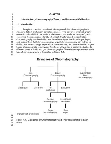
12345678910111213141516171819202122CHAPTER 1Introduction, Chromatography Theory, and Instrument Calibration1.1 IntroductionAnalytical chemists have few tools as powerful as chromatography tomeasure distinct analytes in complex samples. The power of chromatographycomes from its ability to separate a mixture of compounds, or “analytes”, anddetermine their respective identity (chemical structure) and concentration.Chromatography can be divided into three basic types that include gas, liquid,and supercritical fluid chromatography. Liquid chromatography can further bedivided into ion exchange, separations based on size, and even extended to gelbased electrophoretic techniques. This book will provide a basic introduction todifferent types of liquid and gas chromatography. The relationship between eachtype of chromatography is illustrated in Figure 1.1.Figure 1.1. Categories of Chromatography and Their Relationship to EachOther.1
031323334353637383940414243444546In general, each type of chromatography is comprised of two distinctsteps: chromatography (or separation of individual compounds in distinct elutionbands) and identification (detection of each elution band). Gas chromatographyis the process of taking a sample and injecting it into the instrument, turning thesolvent and analytes into gaseous form, and separating the mixture ofcompounds into individual peaks (and preferably individual compounds). Liquidchromatography completes the same process except the separations occur in aliquid phase. Individual band or peaks exit the column and identification occursby a relatively universal detector. One particularly common detector for both gasand liquid chromatography is mass spectrometry (MS) which transforms eachanalyte from a chemically neutral species into a positive cation, usually breakingvarious bonds in the process. Detecting the mass of the individual pieces(referred to as fragments) allows for conclusive identification of the chemicalstructure of the analyte. Principles of gas chromatography (GC) will be coveredin Chapter 2, liquid chromatography (LC) in Chapter 3, capillary electrophoresis(CE) in Chapter 4 and mass spectrometry (MS) in Chapter 5.In mass spectrometry, the combination of compound separation and ionfragment identification (the subject of Chapter 6) yields an extremely powerfulanalysis that is said to be confirmatory. Confirmatory analysis means the analystis absolutely sure of the identity of the analyte. In contrast, many other individualtechniques and detectors are only suggestive, meaning the analyst thinks theyknow the identity of an analyte. This is especially true with most universal GCand LC detectors since these detectors respond similarly to many compounds.The only identifying factor in these chromatographic systems is their elution timefrom the column. In order to obtain confirmatory analysis the sample would needto analyzed by at least two or more techniques (for example, different separationcolumns) that yield the same results. Mass spectrometry and nuclear magneticresonance (NMR) are two confirmatory techniques in chemistry.At this point, it is important to understand the different applications GC-MSand LC-MS offer for two different types of chemists, analytical and syntheticorganic chemists. Organic chemists attempt to create a desired chemicalstructure by transforming functional groups and intentionally breaking or creatingbonds; in their resulting identification procedures they already have a relativelygood idea of the chemical structure. To characterize the resulting product thechemist will use Infrared Spectroscopy (IR) to observe functional groups, MassSpectrometry (MS) to obtain the compound’s molecular weight, and NuclearMagnetic Resonance (NMR) spectroscopy to determine the molecular structure.Information from all three techniques is used to conclusively identify thesynthesized product.Analytical chemists are forced to approach identification in a different way,because they have no a priori knowledge of the chemical structure and becausethe analyte is usually present at low concentrations where IR and NMR areinaccurate. Often, analysis is performed to look for a desired compound by2
0comparing the sample analysis to that of a known (reference) compound. Thereference is used to identify the unknown compound by matching retention time(in chromatography) and ion fragmentation pattern (in mass spectrometry). Withtoday’s computer mass spectral libraries that contain ion fractionation patterns fornumerous chemicals, the analyst has the option of not using a referencestandard. This is especially valuable if a reference compound is not available oris expensive. In some cases, especially with low analyte concentration, thisapproach may only result in a tentative identification.This book will focus on GC-MS and LC-MS applications from an analyticalchemistry perspective even though many synthetic chemists will also find muchof this information useful for their applications.1.2 Chromatographic TheoryAll chromatographic systems have a mobile phase that transports theanalytes through the column and a stationary phase coated onto the column oron the resin beads in the column. The stationary phase loosely interacts witheach analyte based on its chemical structure, resulting in the separation of eachanalyte as a function of time spent in the separation column. The less analytesinteract with the stationary phase, the faster they are transported through thesystem. The reverse is true for less mobile analytes that have strongerinteractions. Thus, the many analytes in a sample are identified by retention timein the system for a given set of conditions. In GC, these conditions include thegas (mobile phase) pressure, flow rate, linear velocity, and temperature of theseparation column. In HPLC, the mobile phase (liquid) pressure, flow rate, linearvelocity, and the polarity of the mobile phase all affect a compounds’ retentiontime. An illustration of retention time is shown in Figure 1.2. The equation at thetop of the figure will be discussed later during our mathematic development ofchromatography theory.31323
739414345474951535557596163656667Figure 1.2. Identification of Analytes by Retention Time.In the above figure, the minimum time that a non-retained chemicalspecies will remain in the system is tM. All compounds will reside in the injector,column, and detector for at least this long. Any affinity for the stationary phaseresults in the compound being retained in the column causing it to elute from thecolumn at a time greater than tM. This is represented by the two larger peaksthat appear to the right in Figure 1.2, with retention times tRA and tRB. CompoundB has more affinity for the stationary phase than compound A because it exitedthe column last. A net retention (tR’A and tR’B) time can be calculated bysubtracting the retention time of the mobile phase(tM) from the peaks retentiontime (tRA and tRB).Figure 1.2 also illustrates how peak shape is related to retention time.The widening of peak B is caused by longitudinal diffusion (diffusion of theanalyte as the peak moves down the length of the column). This relationship isusually the reason why integration by area, and not height, is utilized. However,compounds eluting at similar retention times will have near identical peak shapesand widths.A summary of these concepts and data handling techniques is shown inAnimation 1.1. Click on the figure to start the animation.Animation 1.1. Baseline Resolution.4
0313233343536373839404142Chromatographic columns adhere by the old adage “like dissolves like” toachieve the separation of a complex mixture of chemicals. Columns are coatedwith a variety of stationary phases or chemical coatings on the column wall incapillary columns or on the inert column packing in packed columns. Whenselecting a column’s stationary phase, it is important to select a phasepossessing similar intermolecular bonding forces to those characteristic of theanalyte. For example, for the separation of a series of alcohols, the stationaryshould be able to undergo hydrogen bonding with the alcohols. When attemptingto separate a mixture of non-polar chemicals such as aliphatic or aromatichydrocarbons, the column phase should be non-polar (interacting with theanalyte via van der Waals forces). Selection of a similar phase with similarintermolecular forces will allow more interaction between the separation columnand structurally similar analytes and increase their retention time in the column.This results in a better separation of structurally similar analytes. Specificstationary phases for GC and HPLC will be discussed later in Chapter 2 and 3,respectively.Derivation of Governing Equations: The development of chromatographytheory is a long established science and almost all instrumental texts give nearlyexactly the same set of symbols, equations, and derivations. The derivationbelow follows the same trends that can be found in early texts such as Karger etal. (1973) and Willard et al. (1981), as well as the most recent text by Skoog etal. (2007). The reader should keep two points in mind as they read the followingdiscussion. First, the derived equations establish a relatively simplemathematical basis for the interactions of an analyte between the mobile phase(gas or liquid) and the stationary phase (the coating on a column wall or resinbead). Second, while each equation serves a purpose individually, the relativelylong derivation that follows has the ultimate goal of yielding an equation thatdescribes a way to optimize the chromatographic conditions in order to yieldmaximum separation of a complex mixture of analytes.To begin, we need to develop several equations relating the movement ofa solute through a system to properties of the column, properties of the solute(s)of interest, and mobile phase flow rates. These equations will allow us to predict(1) how long the analyte (the solute) will be in the system (retention time), (2)how well multiple analytes will be separated, (3) what system parameters can bechanged to enhance separation of similar analytes. The first parameters to bemathematically defined are flow rate (F) and retention time (tm). Note that “F” hasunits of cubic volume per time. Retention behavior reflects the distribution of asolute between the mobile and stationary phases. We can easily calculate thevolume of stationary phase. In order to calculate the mobile phase flow rateneeded to move a solute through the system we must first calculate the flow rate.5
1F ( π rc 2 ) ε (L/tm )F π (dc /2)2 ε (L/tm ) π dc F ε (L/tm ) 4 π dc where cross sectional area of column 4 ε porosity of column packing(L/tm ) average linear velocity of mobile 8293031323334In the equations above, rc is the internal column radius, dc is the internal columndiameter, L is the total length of the column, tm is the retention time of a non retained analyte (one which does not have any interaction with the stationaryphase). Porosity (e) for solid spheres (the ratio of the volume of empty porespace to total particle volume) ranges from 0.34 to 0.45, for porous materialsranges from 0.70 to 0.90, and for capillary columns is 1.00. The average linearvelocity is represented by u-bar.The most common parameter measured or reported in chromatography isthe retention time of particular analytes. For a non-retained analyte, we can usethe retention time (tM) to calculate the volume of mobile phase that was neededto carry the analyte through the system. This quantity is designated as Vm,VM tMFmLmin. mL/minEqn 1.1and is called the dead volume. For a retained solute, we calculate the volume ofmobile phase needed to move the analyte through the system by VR tRFEqn 1.2mLmin. mL/minwhere tR is the retention time of the analyte. practice, the analyst does not calculate the volume of theIn actualcolumn, but measures the flow rate and the retention time of non-retained andretained analytes. When this is done, note that the retention time not only is thetransport time through the detector, but also includes the time spent in theinjector! ThereforeVM V column V injector V detectorThe net volume of mobile phase (V’R) required to move a retained analytethrough the system is 6
0313233343536373839VR' VR - VMEqn 1.3where VR is the volume for the retained analyte and VM is the volume for anonretained (mobile) analyte. This can be expanded totR' F tR F - tM Fand dividing by F, yields t' t - tRRMEqn 1.4Equation 1.4 is important since it gives the net time required to move aretained analyte through the system (Illustrated in Figure 1.2, above) Note, for gas chromatography (as opposed to liquid chromatography), theanalyst has to be concerned with the compressibility of the gas (mobile phase),which is done by using a compressibility factor, jwhere Pi is the gas pressure at the inlet of the column and Po is the gas pressureat the outlet. The net retention volume (VN) isVn j VR'Eqn 1.5The next concept that must be developed is the partition coefficient (K)which describes the spatial distribution of the analyte molecules between the mobile and stationaryphases. When an analyte enters the column, it immediatelydistributes itself between the stationary and mobile phases. To understand thisprocess, the reader needs to look at an instant in time without any flow of themobile phase. In this “snap-shot of time” one can calculate the concentration ofthe analyte in each phase. The ratio of these concentrations is called theequilibrium partition coefficient,K Cs / CMEqn 1.6where Cs is the analyte concentration in the solid phase and CM is the soluteconcentration in the mobile phase. If the chromatography system is used over 7
031analyte concentration ranges where the “K” relationship holds true, then thiscoefficient governs the distribution of analyte anywhere in the system. Forexample, a K equal to 1.00 means that the analyte is equally distributed betweenthe mobile and stationary phases. The analyte is actually spread over a zone ofthe column (discussed later) and the magnitude of K determines the migrationrate (and tR) for each analyte (since K describes the interaction with thestationary phase).Equation 1.3 (V’R VR - VM ) relates the mobile phase volume of a nonretained analyte to the volume required to move a retained analyte through thecolumn. K can also be used to describe this difference. As an analyte peak exitsthe end of the column, half of the analyte is in the mobile phase and half is in thestationary phase. Thus, by definitionVR CM VM CM VS CSRearranging and dividing by CM yields V V K VRMSorVR - VM K VSEqn 1.8Now three ways to quantify the net movement of a retained analyte in the columnhave been derived, Equations 1.2, 1.4, and 1.8. Now we need to develop the solute partition coefficient ratio, k’ (alsoknows as the capacity factor), which relates the equilibrium distribution coefficient(K) of an analyte within the column to the thermodynamic properties of thecolumn (and to temperature in GC and mobile phase composition in LC,discussed later). For the entire column, we calculate the ratio of total analytemass in the stationary phase (CSVS) as compared to the total mass in the mobilephase (CMVM), ork' 323334353637383940414243Eqn 1.7CsVsV K sCmVmVmEqn 1.9where VS/VM is sometimes referred to as b, the volumetric phase ratio. Stated in more practical terms, k’ is the additional time (or volume) aanalyte band takes to elute as compared to an unretained analyte divided by theelution time (or volume) of an unretained band, orrearranged, gives8
1357k' t r - tmtm tr tm (1 k' ) 8 91011 121314151617181920212223 L(1 k' )uEqn 1.11Multiple Analytes: The previous discussions and derivations wereconcerned with only one analyte and its migration through a chromatographicsystem. Now we need to describe the relative migration rates of analytes in thecolumn; this is referred to as the selectivity factor, α. Notice Figure 1.2 abovehad two analytes in the sample and the goal of chromatography is to separatechemically similar compounds. This is possible when their distributioncoefficients (Ks) are different. We define the selectivity factor asKBKA k'Bk'AEqn 1.12where subscripts A and B represent the values for two different analytes andsolute B is more strongly retained. By this definition, α is always greater than 1.Also, if one works through the math, you will note thatα 293031323334353637383940Eqn 1.10where µ is the linear gas velocity and the parameters in Equation 1.10 weredefined earlier. So, the retention time of an analyte is related to the partition ratio(k’). Optimal k’ values range from 1 to 5 in traditional packed columnchromatography, but the analysts can use higher values in capillary columnchromatography.α 2425262728Vs - VmVmV'BV'A tR,B - tmtR,A - tm t'R,Bt' R,AEqn 1.13The relative retention time, α, depends on two conditions: (1) the natureof the stationary phase, and (2) the column temperature in GC or the solventgradient in LC. With respect to these, the analyst should always first try to selecta stationary phase that has significantly different K values for the analytes. If thecompounds still give similar retention times, you can adjust the columntemperature ramp in GC or the solvent gradient in LC; this is the general elutionproblem that will be discussed later.Appropriate values of α should range from 1.05 to 2.0 but capillary columnsystems may have greater values.9
1234567891011121314151617Now, we finally reach one of our goals of these derivations, an equationthat combines the system conditions to define analyte separation in terms ofcolumn properties such as column efficiency (H) and the number of separationunits (plates, N) in the column (both of these terms will be defined later). Asanalyte peaks are transported through a column, an individual molecule willundergo many thousands of transfers between each phase. As a result, packetsof analytes and the resulting chromatographic peaks will broaden due to physicalprocesses discussed later. This broadening may interfere with “resolution” (thecomplete separation of adjacent peaks) if their K (or k’) values are close (this willresult in an a value close to 1.0). Thus, the analyst needs a way to quantify acolumn’s ability to separate these adjacent peaks.First, we will start off with an individual peak and develop a concept calledthe theoretical plate height, H, which is related to the width of a solute peak at thedetector. Referring to Figure 1.2, one can see that chromatographic peaks areGaussian in shape, can be described byH 18192021222324252627σLtREqn 1.15Here, L is given in cm and tR in seconds. Note in Figure 1.2, that thetriangulation techniques for determining the base width in time units (t) results in96% if the area or 2 standard deviations, orW 4τ 4343536Eqn 1.14where H is the theoretical plate height (related to the width of a peak as it travelsthrough the column), σ is one standard deviation of the bell-shaped peak, and Lis the column length. Equation 1.14 is a basic statistical way of using standarddeviation to mathematically describe a bell-shaped peak. One standarddeviation on each side of the peak contains 68% of the peak area and it isuseful to define the band broadening in terms of the variance, σ2 (the square ofthe standard deviation, σ). Chromatographers use two standard deviations thatare measured in time units (t) based on the base-line width of the peak, such thatτ 282930313233σ 2LσLtRorσ WL4tREqn 1.16Substitution of Equation 1.16 into Equation 1.14, yields H LW 216t 2 REqn 1.1710
12345678H is always given in units of distance and is a measure of the efficiency ofthe column and the dispersion of a solute in the column. Thus, the lower the Hvalue the better the column in terms of separations (one wants the analyte peakto be as compact as possible with respect to time or distance in the column).Column efficiency is often stated as the number of theoretical plates in a columnof known length, orN 910111213LH tR 2 16 W Eqn 1.18This concept of H, theoretical plates comes from the petroleum distillationindustry as explained in Animation 1.2 below. Click on the Figure to play theanimation. 6263646566Animation 1.2 Origin of H and the Theoretical Plate Height UnitTo summarize Animation 1.2 with respect to gas and liquidchromatography, a theoretical plate is the distance in a column needed toachieve baseline separation; the number of theoretical plates is a way ofquantifying how well a column will perform.11
123456We now have the basic set of equations for describing analyte movementin chromatography but it still needs to be expanded to more practical applicationswhere two or more analytes are separated. Such an example is illustrated inAnimation 1.3 for a packed 51525354555657Animation 1.3 Separation of Two Analytes by Column Chromatography.Separation of two chemically-similar analytes is characterizedmathematically by resolution (Rs), the difference in retention times of theseanalytes. This equation, shown earlier in Figure 1.2, isRs 585960616263642(tR' B - tR' A )WA WBEqn 1.19where tR’B is the corrected retention time of peak B, tR’A is the corrected retentiontime of peak A, WA is the peak width of peak A in time units and WB is the width B. Since WA WB W, Equation 1.19 reduces toof peakRs 65 tR' B - tR' AWEqn 1.2012
123Equation 1.18 expressed W in terms of N and tR, and substitution of Equation1.17 into Equation 1.18, yields t- tR' A NRs R' B tR' B 445Eqn 1.21Recall from Equation 1.10, that 678substitution into Equation 1.21 and upon rearrangement, yieldsRs9101112131416182021222426283031323334 k'- k'A B 1 k'B N4Eqn 1.22Recall that we are trying to develop an equation that relates resolution torespective peak separations and although k’ values do this, it is more useful to expressthe equation in terms of α, where α k’B/k’A. Substitution of α intoEquation 1.22, with rearrangement, yieldsRs α - 1 k'Bα 1 k'BN4Eqn 1.23or the analyst can determine the number of plates required for a givenseparation: 2 k'B 22 α - 1 N 16 Rs Eqn 1.24 α 1 k'B Thus, the number of plates present in a column can be determined by directinspection of a chromatogram, where Rs is determined from Equation 1.20, k’Aand k’ B are determined using Equation 1.10, and α is determined using Equation1.12.Rs k’3536 tR,B - tR,AWt r - tmtm Vs - VmVmEqn 1.20Eqn 1.10 α KBKA k'Bk'AEqn 1.1213
1234567891011121314151617181920212223Another use of Equation 1.23 is that it can be used to explain improvedseparation with temperature programming of the column in GC and gradientprogramming in HPLC. Recall that poorer separation will result as peaksbroaden as they stay for extended times in the column and several factorscontribute to this process. N can be changed by changing the length of thecolumn to increase resolution but this will further increase band broadening. Hcan be decreased by altering the mobile phase flow rate, the particle size of thepacking, the mobile phase viscosity (and thus the diffusion coefficients), and thethickness of the stationary phase film.To better understand the application of the equations derived above auseful exercise is to calculate all of the column quantification parameters for aspecific analysis. The chromatogram below (Figure 1.3) was obtained from acapillary column GC with a flame ionization detector. Separations ofhydrocarbons commonly found in auto petroleum were made on a 30-meter long,0.52-mm diameter DB-1 capillary column. Table 1.1 contains the output from atypical integrator.Figure 1.3 Integrator Output for the Separation of Hydrocarbons by CapillaryColumn GC-FID.14
12Table 1.1 Integrator Output for the Chromatogram shown in Figure 1.3.AnalyteSolvent (tM)BenzeneIso-octanen-HeptaneTolueneEthyl Benzeneo-Xylenem-Xylene345678910Retention Peak Width at theBase (in units mple 1.1Calculate k’, α, Rs, H, and N for any two adjacent compounds in Table 1.1.Solution:Using peaks eluting at 13.724 and 13.359 minutes the following valueswere obtained.1112131415161718Problem 1.1Figure 1.4 and Table 1.2 contain data from an HPLC analysis of four s-Triazines(common herbicides). Calculate k’, α, Rs, H, and N for any two adjacentcompounds. Compare and contrast the results for the resin packed HPLCcolumn to those of the capillary column in the GC example given above.15
12345678Figure 1.4 HPLC Chromatogram of Four Triazines. The analytical column wasan 10.0 cm C-18 stainless steel column with 2 µm resin beads.Table 1.2 Integrator Output for the HPLC Chromatogram shown in Figure 1.4.AnalyteSolvent (tM)Peak 1Peak 2Peak 3Peak 491011121314151617181920Retention 175515053811476639Peak Width at theBase (in units ofminutes)NA0.1910.2060.2060.1981.3 Optimization of Chromatographic ConditionsNow we will review and summarize this lengthy derivation and thesecomplicated concepts. Optimization of the conditions of the chromatographysystem (mobile phase flow rate, stationary phase selection, and columntemperature or solvent gradient) are performed to achieve base-line resolutionfor the most difficult separation in the entire analysis (two adjacent peaks). Thisprocess results in symmetrically-shaped peaks that the computer can integrate toobtain a peak (analyte) area or peak height. A series of known referencestandards are used to generate a linear calibration line (correlating peak area or16
12345678910111213141516171819202122232425height to analyte concentration) for each compound. This line, in turn, is used toestimate the concentration of analyte in unknown samples based on peak area orheight.An instrument’s resolution can be altered by changing the theoretical plateheight and the number of theoretical plates in a column. The plate height, asexplained in the animation below, is the distance a compound must travel in acolumn needed to separation two similar analytes. The number of theoreticalplates in a column is a normalized measure of how well a column will separatesimilar analytes.Now it is necessary to extend the concept of theoretical plate height (H) abit further to understand its use in chromatography. Since gas and liquidchromatography are dynamic systems (mobile flow through the column), it isnecessary to relate a fixed length of the column (the theoretical plate height) toflow rate in the column. Flow rate is measured in terms of linear velocity, or howmany centimeters a mobile analyte or carrier gas will travel in a given time(cm/s). The optimization of the relationship between H and linear velocity (µ),referred to as a van Deemter plot, is illustrated in Figure 1.5 for gaschromatography.Figure 1.5. A Theoretical van Deemter Plot for a Capillary Column showing theRelationship between Theoretical Plate Height and Linear Velocity.17
1234567891011121314It is desirable to have the smallest plate height possible, so the maximumnumber of plates can be “contained” in a column of a given length. Three factorscontribute to the effective plate height, H, in the separation column. The first isthe longitudinal diffusion, B (represented by the blue line in Figure 1.5) of theanalytes that is directly related to the time an analyte spends in the column.When the linear velocity (µ) is high, the analyte will only spend a short time in thecolumn and the resulting plate height will be small. As linear velocity slows, morelongitudinal diffusion will cause more peak broadening resulting in lessresolution. The second factor is the multi-flow path affect represented by the redline in Figure 1.5. This was a factor in packed columns but has been effectivelyeliminated when open tubular columns (capillary columns) became the industrystandard. Third are the limitations of mass transfer between and within the gasand stationary phases, Cu (the yellow line in Figure 3) defined e µ is the mobile phase linear velocity, Ds and Dm are diffusion coefficients inthe stationary and mobile phases respectively, df and dp are the diameter of thepacking particles and the thickness of liquid coating on the stationary phaseparticles respectively, k is the unitless retention or capacity factor, and f(k) andf’(k) are mathematical functions of k.If the linear velocity of the mobile phase is too high, the entire “packet” of agiven analyte will not have time to completely transfer between the mobile andstationary phase or have time to completely move throughout a given phase(phases are coated on the column walls and therefore have a finite thickness).This lack of complete equilibrium of the analyte molecules will result in peakbroadening for each peak or skewing of the Gaussian shape. This, in turn, willincrease H and decrease resolution.The green line in Figure 1.5 represents the van Deemter curve, thecombined result of the three individual phenomena. Since the optimum operatingconditions has the smallest plate height; the flow rate of the GC should be set tothe minimum of the van Deemter curve. For gas chromatography this occursaround a linear velocity of 15 to 20 cm/s. However, in older systems, as the ovenand column were temperature programmed, the velocity of the gas changed18
1234568101214161820
10 This book will focus on GC-MS and LC-MS applications from an analytical 11 chemistry perspective even though many synthetic chemists will also find much 12 of this information useful for their applications. 13 14 1.2 Chromatographic Theory 15 16 All chroma