Transcription
NASA TECHNICALNOTENASA TN D-7770A STREAMLINE CURVATURE METHODFOR DESIGN OF SUPERCRITICALAND SUBCRITICAL AIRFOILSOCT 2 !) 1974by Raymond L. Barger and Cuyler W. Brooks,Langley Research CenterHampton, Va. 23665NATIONAL AERONAUTICS AND SPACE ADMINISTRATION WASHINGTON, D. C. SEPTEMBER 1974
1. Report No.2. Government Accession No.3. Recipient's Catalog No.NASA TN D-77704. Title and Subtitle5. Report DateSeptember 1974A STREAMLINE CURVATURE METHOD FOR DESIGN OFSUPERCRITICAL AND SUBCRITICAL AIRFOILS6. Performing Organization Code7. Author(s)8. Performing Organization Report No.L-9747Raymond L. Barger and Cuyler W. Brooks, Jr.10. Work Unit No.9. Performing Organization Name and Address501-06-05-08NASA Langley Research CenterHampton, Va. 2366511. Contract or Grant No.13. Type of' Report and Period Covered12. Sponsoring Agency Name and AddressTechnical NoteNational Aeronautics and Space AdministrationWashington, D.C. 2054614. Sponsoring Agency Code15. Supplementary Notes16. AbstractAn airfoil design procedure, applicable to both subcritical and supercritical airfoils,is described. The method is based on the streamline curvature velocity equation. Severalexamples illustrating this method are presented and discussed.17. Key Words (Suggested by Author(s))18. Distribution StatementUnclassified - UnlimitedAirfoilDesignSupercriticalStreamline curvature19. Security dassif. (of this report!UnclassifiedSTAR Category 0120. Security Classif. (of this page)Unclassified21. No. of Pages22. Price*14For sale by the National Technical Information Service, Springfield, Virginia 22151 3.00
A STREAMLINE CURVATURE METHOD FOR DESIGN OFSUPERCRITICAL AND SUBCRITICAL AIRFOILSBy Raymond L. Barger and Cuyler W. Brooks, Jr.Langley Research CenterSUMMARYAn airfoil design procedure, applicable to both subcritical and supercritical airfoils,is described. The method is based on the streamline curvature velocity equation. Several examples illustrating this method are presented and discussed.INTRODUCTIONA number of airfoil design methods are currently in existence. Most of these areconfined within the framework of incompressible flow analysis. (See refs. 1 to 3 andthe references therein.) Interest in supercritical airfoil sections has led to the development of compressible flow design procedures, such as those described in references 4and 5.- .The method described in this paper is also a compressible flow method but differsin some essential respects from the latter two analyses. First, it designs the airfoilfrom a prescribed pressure distribution rather than from a set of parameters. Thisfeature enables one to design airfoils which are relatively insensitive to variations fromthe design conditions, since some types of pressure distributions have less tendency thanothers to develop shocks with small changes in Mach number or angle of attack. Thismethod also permits the designer to work directly with the pressure distribution to alterperformance parameters such as pitching moment.Another advantage of the present method is that the calculations are performed inthe physical plane rather than in the hodograph plane, and the pressure variations arerelated directly to the airfoil geometry. Thus, the designer has a physically intuitiveinsight into the nature of the variations at each stage in the design process.Application of the method requires an initial airfoil with a pressure distribution thatroughly approximates the desired one. The pressure distribution obtained is generallynot exactly the one specified but is a significantly closer approximation than that of theunmodified airfoil.
The method described is implemented through a series of computer programs whichshare the common feature of being based on the analysis program of reference 6. Thisanalysis program is used in successive modifications of the airfoil contour until thedesired result is obtained.There is no guarantee that, at some given angle of attack and Mach number, anarbitrary modification in the pressure distribution on the airfoil can be obtained by anypractical modification of the contour. Only extensive use will reveal the actual limitations of the method.SYMBOLSastreamline curvatureCempirical parametercairfoil chord lengthcairfoil pitching-moment coefficient about the quarter-chord pointcairfoil pressure coefficientkconstantMMach numberndistance in direction normal to streamlinesPpoint on airfoil surfaceqlocal velocityRlocal radius of curvaturetairfoil thicknessx,yairfoil coordinates
Subscripts:iith pointsconditions at airfoil surface00conditions at infinityANALYSISBasic ConsiderationsThe design procedure requires as a starting point an airfoil of known contour.Convergence is improved if the characteristics of this airfoil approximate the desiredcharacteristics. The pressure distribution of the initial airfoil need not be known withaccuracy inasmuch as it is computed in the first phase of the design process. Aerodynamic characteristics of the new airfoil design are controlled by the specification of adesired pressure distribution which may display a considerable degree of arbitrariness.All the practical airfoil problems encountered thus far in applying this method have beenin tailoring the pressure distribution of a given airfoil for which the performance hadbeen somewhat unsatisfactory. Some examples of specified alterations are(1) Altering the inviscid upper surface shock structure at a supercritical Machnumber to decrease the adverse shock effects(2) Increasing the upper surface suction near the nose and decreasing it at the crest" to obtain a higher drag divergence Mach number at low angles of attack(3) Decreasing the upper surface velocity near the nose to obtain better performanceat high angles of attack(4) Shifting the loading from the aft region toward the middle to decrease the magnitude of the pitching momentCalculation ProcedureThe design calculation proceeds according to the following steps:(1) Compute the pressure distribution of the initial airfoil by the method ofreference 6.(2) Compute the difference between this pressure distribution and the desireddistribution.
(3) Compute an airfoil variation, based on this difference, with a pressure distribution closer to that desired.(4) Iterate: Replace the initial airfoil with the variation obtained in step (3).This process is terminated by prescribing the number of iterations. It is not practicalto prescribe a maximum error, inasmuch as it is not known initially how closely theprescribed distribution can be approximated.Calculation of Airfoil ChangeStep (3) in the preceding section requires a mathematical expression relating achange in the airfoil contour to a change in the pressure distribution. This expressioncan be a perturbation type of expression, inasmuch as it represents a relation betweenvariations or increments. Furthermore, it need not be extremely accurate because theiteration process will generally improve the approximation.To obtain such an expression, one may start with the momentum equation in thestreamline curvature form. This equation gives, for the velocity distribution along astreamline normal,f1 - -a(n) dn.(1)In equation (1) the curvature a of a streamline is simply the reciprocal of its local radius of curvature. Consider a point on the airfoil surface where the local curvature isa0s. The streamlines transversed by a normal emanating from this point have curvaturea o at the surface and curvature approaching zero as n approaches infinity (in subsonicflow). This curvature distribution is arbitrarily assumed to have a negative exponentialforma(n) a -1 (2)for some k which is constant for a given normal but may vary from one normal toanother.Such a variation is certainly a reasonable approximation for those normals thatemanate from points near the crest of the airfoil. At the surface where n 0, a aand the curvature of the streamlines rapidly decreases as n increases. On the otherhand, the curvature decrease along normals emanating, say near the leading edge, isclearly not exponential, since the curvature distribution along these normals changessign. One is motivated, however, to explore the possibility of applying equation (2) overthe entire airfoil for several reasons:
(1) Since only the values at the surface are required, the importance of the incorrect curvature variation away from the surface is minimized.(2) As a result of assuming equation (2), a relation between the surface geometryand the surface velocity can be obtained without a calculation of the entire flow field.(3) The parameter k, which may vary along the surface, can be varied to providesome compensation for the error involved in the assumed form of the curvature variation.Therefore, proceeding to explore the use of equation (2), one substitutes equation(2) into equation (1) and integrates the resulting equation outward along a normal. Thus,f - k n , -ao \ edn o-Qr \JJS qwhich results in the relationa Now, if one postulates a small local variation in surface curvature Aa ,s theresulting change in q0o is obtained from equation (3) asAqAassIf the parameter k in equation (4) is obtained from equation (3), the result isAqsqAas ins "asor, if the change in velocitycurvature isAq5 is specified, the corresponding increment in surface(5)
It is necessary to examine this expression in some detail. Near the crest of the airfoilwhere q q , the logarithm varies gradually, and the expression gives a near proportion between AaS//a S and AqS//q S . On the other hand, where aS qTO (that is, wherethe pressure coefficient is zero) the logarithm is zero, and the expression becomesunusable. This problem arises because of the error involved in the assumption of equation (2). However, there is no physical reason why the flow at the surface should bequalitatively different at a point where c 0 than at any other point. Therefore, thepossibility exists, as suggested earlier, of altering the parameter k to compensate forthe error involved in assuming the exponential variation in equation (2) 0 The most obviouspossibility is to setk Caswhich will give a simple proportion between AaS//a S and AqS//qS everywhere on theairfoil. Equation (5) is replaced with an equation of the formAas Cas- 6 which gives a variation approximately similar to equation (5) where qg q and a muchmore reasonable variation where q q . Thus C is an empirical parameter whichis, in general, a function of local Mach number or of local curvature. In actual practiceit has been found to be sufficient to let C vary with free-stream Mach number. A valuethat is often used initially isC*lo(l If the step size on each iteration then appears to be too large or too small, C is adjustedaccordingly. Normally, no more than one such adjustment is required.Airfoil Profile ModificationThe curvature distribution of the modified airfoil is known from the curvature distribution of the original airfoil plus the change in curvature given by equation (6]L Theprofile coordinates can then be computed by using simple geometric concepts, such asthe fact that a circle is determined by any three noncollinear points on its circumferenceor by its radius and two points on the circumference.If the modification is to the upper surface, the new contour is constructed as follows: If Pj denotes the first point of the prescribed region of change, then a circleis determined which contains PJ J and P, on the airfoil and has radius R 7p6
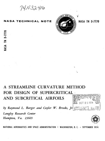
(See fig. l(a).) At the next specified x-location, the y-coordinate of a point on this circleis found. This x,y pair represents the coordinates on the new contour which now has thedesired curvature at P. The next point P i 2 is now constructed so that the contourwill have the prescribed curvature at Pi i- This procedure is continued, with the useof the new curvature distribution, to the end of the region of change. Then it is continuedto the trailing edge, with the use of the curvature distribution of the original airfoil inthis region.The trailing-edge point of the new contour computed in this manner will usually beabove or below the trailing edge of the original airfoil. The resulting gap is closed witha linear adjustment starting at the leading edge. (See fig. l(b).) Since this adjustmentalters the ordinates linearly, it changes the slopes by a constant and leaves the curvaturedistribution unchanged between the leading edge and the trailing edge. This adjustmentchanges the pressure distribution somewhat outside of the prescribed region of changeand results in a generally small distributed error there.If the modification is prescribed for the lower surface instead of the upper surface,a similar procedure is followed. However, since the calculation proceeds from thetrailing edge to the leading edge along the lower surface, the gap must be closed at theleading edge instead of the trailing edge.The examples shown in figures 2, 3, and 4 were computed by use of the methodjust discussed. However, an alternative method of handling the discontinuity at the endof the region for which changes in the local radius of curvature are specified was usedin some cases. The gap in the coordinates at this point was closed by a linear transformation pivoted at the first point of the region. This method left discontinuities in theslope at the end points of the region of change, but these were eliminated by a simplefairing algorithm. This alternative method was used to generate the final curve of figure 5, and it can be seen that no discontinuities appear at the end points of the region ofchange, 5.3 percent and 92.6 percent of the profile chord.Boundary-Layer ConsiderationsAlthough the procedure described is an inviscid calculation, some allowance for theboundary layer can be made. One way of doing this would be to perform the calculationfor a composite profile consisting of the basic airfoil plus its boundary-layer displacement thickness. In the design process, the trailing-edge thickness would be adjusted tojust equal the original boundary-layer displacement thickness. After the completion ofthe design, the original boundary-layer displacement thickness would be subtracted togive the actual airfoil ordinates. For this approximation, the boundary layers on theoriginal and modified airfoils are assumed to be essentially the same.
An alternate procedure would be as follows:(1) Calculate both the viscous and inviscid pressure distributions for both airfoils.(2) Specify the desired viscous pressure distribution and obtain the differencebetween the original and desired viscous distributions.(3) Specify the desired inviscid distribution as the original inviscid pressure plusthe difference obtained in step (2).(4) Obtain the resulting design and compute its viscous pressure distribution. Ifthe viscous pressure distribution on the new airfoil is not sufficiently close to that desired,the process can be iterated.A third possibility, of course, would be to replace the inviscid analysis phase ofthe iteration process with a calculation that includes the boundary layer.EXAMPLESThe first example, shown in figure 2, illustrates a modification to the upper surface of a supercritical airfoil, intended to decrease the leading-edge suction peak and toincrease the suction somewhat aft of the peak. It is seen that, with two iterations, thedesired distribution is obtained approximately. This type of change results in a somewhat thicker airfoil.The second example (fig. 3) represents a more practical problem. It shows a modification to the lower surface designed to decrease the pitching moment without decreasingthe lift. The thinning of the airfoil is a result of increasing the loading in the middle portion of the lower surface. Such a change could be combined with that of the first exampleto compensate for the thickening tendency of that type of modification. For this particular modification, the prescribed change was almost exactly obtained.The third example (fig. 4) shows a different type of modification to the original airfoil used in the first example. This example has two complicating factors. First, theairfoil is designed for performance at an angle of attack of 2 . Second, the pressure distribution of the original airfoil contains a fairly strong shock wave within the prescribedregion of change. After three iterations, the pressure distribution obtained still deviatessomewhat from the desired distribution, especially in the vicinity of the leading-edge suction peak; but the extreme velocities have been reduced, the shock ceases to be a problem,and the desired distribution is closely approximated over most of the airfoil.In this example, the thickening of the airfoil is significant. As a matter of fact, ifthe iteration process were continued to reduce the discrepancy near the leading edge further, an even thicker airfoil would result. Not all significant modifications in the pressure8
distribution result in significant thickness changes, however, as is demonstrated in thenext example.The fourth example, illustrated in figure 5, involves a large region of supersonicflow on the upper surface. The problem was to replace a pressure distribution havingtwo moderately strong shock waves with one having a single weak wave, and the desiredpressure distribution was nearly obtained after six iterations, as shown in the figure.No attempt was made to retain the original lift coefficient, and the lift coefficient of themodified profile is slightly lower. As mentioned previously, the change in thickness ratiowas insignificant.CONCLUDING REMARKSAn airfoil design procedure applicable to both subcritical and supercritical airfoilshas been described. The method is based on the streamline curvature velocity equation.This method does not include the boundary-layer calculation directly, but suggestions forapplying the method to the viscous case were given. Several examples illustrating thismethod were presented and discussed.Langley Research Center,National Aeronautics and Space Administration,Hampton, Va., August 14, 1974.REFERENCES1. Barger, Raymond L.: A Modified Theodorsen e-Function Airfoil Design Procedure.NASA TND-7741, 1974.2. Strand, T.: Exact Method of Designing Airfoils With Given Velocity Distribution inIncompressible Flow. J. Aircraft, vol. 10, no. 11, Nov. 1973, pp. 651-659.3. James, Richard M.: A General Class of Exact Airfoil Solutions. J. Aircraft, vol. 9,no. 8, Aug. 1972, pp. 574-580.4. Garabedian, P. R.; and Korn, D. G.: Numerical Design of Transonic Airfoils. Numerical Solution of Partial Differential Equations - n, Bert Hubbard, ed., AcademicPress,Inc., 1971, pp. 253-271.5. Nieuwland, G. Y.: Theoretical Design of Shock-Free, Transonic Flow Around Aerofoil Sections. Aerospace Proceedings 1966, Vol. 1, Joan Bradbrooke, Joan Bruce,and Robert R. Dexter, eds., Macmillan and Co., Ltd., c.1967, pp. 207-240.6. Garabedian, P. R.; and Korn, D. G.: Analysis of Transonic Airfoils. Commun. Pure& Appl. Math., vol. 24, no. 6, Nov. 1971, pp. 841-851.9
Original(Center at arc pT7 Pjl i e s onperpendicular bisector ofchord P\ \ P\ }(a) Method of defining revised ordinates.Upper surface after revising ordinatesTrailingedgeLinear adjustmentAdjusted upper surface(b) Method of correcting trailing-edge closure.Figure 1.- Illustration of methods used in the definition ofredesigned airfoil sections.10
-2.0r- 1.5M 1.0 —OriginalPrescribedActually obtained-1.0- .50.51.01.5LOriginal, t/c 0.110Modified, t/c 0.116Figure 2.- Compressible flow design method applied to a supercritical airfoilat zero angle of attack. M 0.6; two iterations.11
-1-5-1.0OriginalCn0-0/Actually obtained".51-01.5Original, t/c .095, c m -.Q25Modified, t/c. .090, cm -.010Figure 3.- Modification to lower surface designed to decrease pitching momentwithout decreasing lift. M 0.75; angle of attack 0.8; five iterations.12
-2.5r-2.0-M 1.46-OriginolA c t u a l l y obtainedPrescribed- 1.5M 1.0 —- 1.0.5Cp0.51.01.5LOriginal, t/c 0.110Modified, t/c 0.124Figure 4.- Compressible flow design method applied to a supercritical airfoilat 2 angle of attack. 1VL, 0.6; three iterations.XL3
-1.5r-1.0PrescribedActuallyobtained -0.5-c P00.51.0i.51-Original, t/c 0.110Modified, t/c 0.110Figure 5.- Compressible flow design method applied to a supercritical airfoilat zero angle of attack. M 0.75; six iterations.14NASA-Langley, 1974L-9747
NATIONAL AERONAUTICS AND SPACE ADMINISTRATIONWASHINGTON. D.C. 2O546POSTAGE AND FEESPAIDNATIONAL AERONAUTICS ANDOFFICIAL BUSINESSPENALTY FOR PRIVATE USE 3OOSPACE ADMINISTRATIONSPECIAL FOURTH-CLASSBOOKRATE451AEROHOI.BOSIC DIVAEROSPACE 6 COHMDNICATIONS OPERATIONSATTN: TECHHICAL 1TNFO SERVICESFORD S JAMBOBBE ROADSNEWPORT BEACH CA 92663POSTMASTER :If Tjndeliverable (Section 158Postal Manual) Do Not Return"The aeronautical and space activities of the United States shall beconducted so as to contribute . . . to the expansion of human knowledge of phenomena in the atmosphere and space. The Administrationshall provide for the widest practicable and appropriate disseminationof information concerning its activities and the results thereof."—NATIONAL AERONAUTICS AND SPACE ACT OF 1958NASA SCIENTIFIC AND TECHNICAL PUBLICATIONSTECHNICAL REPORTS: Scientific andtechnical information considered important,complete, and a lasting contribution to existingknowledge.TECHNICAL TRANSLATIONS: Informationpublished in a foreign language consideredto merit NASA distribution in English.TECHNICAL NOTES: Information less broadin scope but nevertheless of importance as acontribution to existing knowledge.SPECIAL PUBLICATIONS: Informationderived from or of value to NASA activities.Publications include final reports of majorprojects, monographs, data compilations,handbooks, sourcebooks, and specialbibliographies.TECHNICAL MEMORANDUMS:Information receiving limited distributionbecause of preliminary data, security classification, or other reasons. Also includes conferenceproceedings with either limited or unlimiteddistribution.CONTRACTOR REPORTS: Scientific andtechnical information generated under a NASAcontract or grant and considered an importantcontribution to existing knowledge.TECHNOLOGY UTILIZATIONPUBLICATIONS: Information on technologyused by NASA that may be of particularinterest in commercial and other non-aerospaceapplications. Publications include Tech Briefs,tt Technology Utilization Reports andv Technology Surveys.Details on fhe availability of fhese pubf/cafions may be obtained from:SCIENTIFIC AND TECHNICAL INFORMATION OFFICENATIONALAERONAUTICSANDSPACEWashington, D.C. 20546ADMINISTRATION
streamline curvature form. This equation gives, for the velocity distribution along a streamline normal, f1--a(n) dn . (1) In equation (1) the curvature a of a streamline is simply the reciprocal of its local rad-ius of curvature. Consider a point on the airfoil surface where the local curv