Transcription
ECE 380: Control SystemsCourse Notes: Winter 2014Prof. Shreyas SundaramDepartment of Electrical and Computer EngineeringUniversity of Waterloo
iic Shreyas Sundaram
AcknowledgmentsParts of these course notes are loosely based on lecture notes by ProfessorsDaniel Liberzon, Sean Meyn, and Mark Spong (University of Illinois), on notesby Professors Daniel Davison and Daniel Miller (University of Waterloo), andon parts of the textbook Feedback Control of Dynamic Systems (5th edition) byFranklin, Powell and Emami-Naeini. I claim credit for all typos and mistakesin the notes.The LATEX template for The Not So Short Introduction to LATEX 2ε by T. Oetikeret al. was used to typeset portions of these notes.Shreyas SundaramUniversity of Waterlooc Shreyas Sundaram
ivc Shreyas Sundaram
Contents1 Introduction11.1Dynamical Systems . . . . . . . . . . . . . . . . . . . . . . . . . .11.2What is Control Theory? . . . . . . . . . . . . . . . . . . . . . .21.3Outline of the Course . . . . . . . . . . . . . . . . . . . . . . . .42 Review of Complex Numbers53 Review of Laplace Transforms93.1The Laplace Transform . . . . . . . . . . . . . . . . . . . . . . .93.2The Inverse Laplace Transform . . . . . . . . . . . . . . . . . . .133.2.1Partial Fraction Expansion . . . . . . . . . . . . . . . . .13The Final Value Theorem . . . . . . . . . . . . . . . . . . . . . .153.34 Linear Time-Invariant Systems174.1Linearity, Time-Invariance and Causality . . . . . . . . . . . . . .174.2Transfer Functions . . . . . . . . . . . . . . . . . . . . . . . . . .184.2.14.3Obtaining the transfer function of a differential equationmodel . . . . . . . . . . . . . . . . . . . . . . . . . . . . .20Frequency Response . . . . . . . . . . . . . . . . . . . . . . . . .215 Bode Plots5.125Rules for Drawing Bode Plots . . . . . . . . . . . . . . . . . . . .265.1.127Bode Plot for Ko . . . . . . . . . . . . . . . . . . . . . . .q5.1.2Bode Plot for s. . . . . . . . . . . . . . . . . . . . . . .285.1.3Bode Plot for ( ps 1) 1 and ( zs 1) . . . . . . . . . . . .29c Shreyas Sundaram
viCONTENTS5.1.4 1 . . . . . . . . . . .Bode Plot for ( ωsn )2 2ζ( ωsn ) 1325.1.5Nonminimum Phase Systems . . . . . . . . . . . . . . . .346 Modeling and Block Diagram Manipulation6.16.237Mathematical Models of Physical Systems . . . . . . . . . . . . .376.1.1Mechanical Systems . . . . . . . . . . . . . . . . . . . . .376.1.2Electrical Systems . . . . . . . . . . . . . . . . . . . . . .386.1.3Rotational Systems . . . . . . . . . . . . . . . . . . . . . .39Block Diagram Manipulation . . . . . . . . . . . . . . . . . . . .416.2.145Systems with Multiple Inputs and Outputs . . . . . . . .7 Step Responses of Linear Systems7.17.247Step Response of First Order Systems . . . . . . . . . . . . . . .477.1.1Rise time . . . . . . . . . . . . . . . . . . . . . . . . . . .487.1.2Settling time . . . . . . . . . . . . . . . . . . . . . . . . .49Step Response of Second Order Systems . . . . . . . . . . . . . .507.2.1Underdamped and Critically Damped Systems (0 ζ 1) 507.2.2Overdamped System (ζ 1) . . . . . . . . . . . . . . . .527.2.3Discussion . . . . . . . . . . . . . . . . . . . . . . . . . . .528 Performance of Second Order Step Responses8.155Performance Measures . . . . . . . . . . . . . . . . . . . . . . . .558.1.1Rise time (tr ) . . . . . . . . . . . . . . . . . . . . . . . . .568.1.2Peak value (Mp ), Peak time (tp ) and Overshoot OS . . .568.1.3Settling Time (ts ) . . . . . . . . . . . . . . . . . . . . . .578.2Choosing Pole Locations to Meet Performance Specifications . .588.3Effects of Poles and Zeros on the Step Response . . . . . . . . . .608.3.1Effect of a Zero on the Step Response . . . . . . . . . . .618.3.2Effect of Poles on the Step Response . . . . . . . . . . . .639 Stability of Linear Time-Invariant Systems659.1Pole-zero cancellations and stability . . . . . . . . . . . . . . . .659.2Stability of the Unity Feedback Loop . . . . . . . . . . . . . . . .679.3Tests for Stability . . . . . . . . . . . . . . . . . . . . . . . . . . .68c Shreyas Sundaram
CONTENTSvii9.3.1A Necessary Condition for Stability . . . . . . . . . . . .9.3.2A Necessary and Sufficient Condition: Routh-Hurwitz Test 709.3.3Testing For Degree of Stability . . . . . . . . . . . . . . .729.3.4Testing Parametric Stability with Routh-Hurwitz . . . . .7310 Properties of Feedback687510.1 Feedforward Control . . . . . . . . . . . . . . . . . . . . . . . . .7610.2 Feedback Control . . . . . . . . . . . . . . . . . . . . . . . . . . .7711 Tracking of Reference Signals8111.1 Tracking and Steady State Error . . . . . . . . . . . . . . . . . .12 PID Control12.1 Proportional (P) Control8289. . . . . . . . . . . . . . . . . . . . . .8912.2 Proportional-Integral (PI) Control . . . . . . . . . . . . . . . . .9112.3 Proportional-Integral-Derivative (PID) Control . . . . . . . . . .9112.4 Implementation Issues . . . . . . . . . . . . . . . . . . . . . . . .9313 Root Locus9513.1 The Root Locus Equations . . . . . . . . . . . . . . . . . . . . .9713.1.1 Phase Condition . . . . . . . . . . . . . . . . . . . . . . .9813.2 Rules for Plotting the Positive Root Locus . . . . . . . . . . . . . 10013.2.1 Start Points and (Some) End Points of the Root Locus. 10013.2.2 Points on the Real Axis . . . . . . . . . . . . . . . . . . . 10013.2.3 Asymptotic Behavior of the Root Locus . . . . . . . . . . 10113.2.4 Breakaway Points . . . . . . . . . . . . . . . . . . . . . . . 10513.2.5 Some Root Locus Plots . . . . . . . . . . . . . . . . . . . 10813.2.6 Choosing the Gain from the Root Locus . . . . . . . . . . 11013.3 Rules for Plotting the Negative Root Locus . . . . . . . . . . . . 11114 Stability Margins from Bode Plots11515 Compensator Design Using Bode Plots12315.1 Lead and Lag Compensators . . . . . . . . . . . . . . . . . . . . 12315.2 Lead Compensator Design . . . . . . . . . . . . . . . . . . . . . . 12615.3 Lag Compensator Design . . . . . . . . . . . . . . . . . . . . . . 130c Shreyas Sundaram
viiiCONTENTS16 Nyquist Plots13516.1 Nyquist Plots . . . . . . . . . . . . . . . . . . . . . . . . . . . . . 13816.2 Drawing Nyquist Plots . . . . . . . . . . . . . . . . . . . . . . . . 14016.2.1 Nyquist Plots For Systems With Poles/Zeros On The Imaginary Axis . . . . . . . . . . . . . . . . . . . . . . . . . . . 14316.3 Stability Margins from Nyquist Plots . . . . . . . . . . . . . . . . 14617 Modern Control Theory: State Space Models15117.1 State-Space Models . . . . . . . . . . . . . . . . . . . . . . . . . . 15117.2 Nonlinear State-Space Models and Linearization . . . . . . . . . 15617.2.1 Linearization via Taylor Series . . . . . . . . . . . . . . . 15717.3 The Transfer Function of a Linear State-Space Model . . . . . . 15917.4 Obtaining the Poles from the State-Space Model . . . . . . . . . 16017.5 An Overview of Design Approaches for State-Space Models . . . 162c Shreyas Sundaram
Chapter 1Introduction1.1Dynamical SystemsFor the purposes of this course, a system is an abstract object that accepts inputsand produces outputs in response. Systems are often composed of smaller components that are interconnected together, leading to behavior that is more thanjust the sum of its parts. In the control literature, systems are also commonlyreferred to as plants or processes.InputSystemOutputFigure 1.1: An abstract representation of a system.The term dynamical system loosely refers to any system that has an internalstate and some dynamics (i.e., a rule specifying how the state evolves in time).This description applies to a very large class of systems, from automobiles andaviation to industrial manufacturing plants and the electrical power grid. Thepresence of dynamics implies that the behavior of the system cannot be entirely arbitrary; the temporal behavior of the system’s state and outputs can bepredicted to some extent by an appropriate model of the system.Example 1. Consider a simple model of a car in motion. Let the speed ofthe car at any time t be given by v(t). One of the inputs to the system is theacceleration a(t), applied by the throttle. From basic physics, the evolution ofthe speed is given bydv a(t).(1.1)dtThe quantity v(t) is the state of the system, and equation (1.1) specifies thedynamics. There is a speedometer on the car, which is a sensor that measuresc Shreyas Sundaram
2Introductionthe speed. The value provided by the sensor is denoted by s(t) v(t), and thisis taken to be the output of the system.As shown by the above example, the inputs to physical systems are applied viaactuators, and the outputs are measurements of the system state provided bysensors.Other examples of systems: Electronic circuits, DC Motor, Economic Systems, . . .1.2What is Control Theory?The field of control systems deals with applying or choosing the inputs to agiven system to make it behave in a certain way (i.e., make the state or outputof the system follow a certain trajectory). A key way to achieve this is via theuse of feedback, where the input depends on the output in some way. This isalso called closed loop control.InputSystemOutputMapping fromoutput to inputFigure 1.2: Feedback Control.Typically, the mapping from outputs to inputs in the feedback loop is performedvia a computational element known as a controller, which processes the sensormeasurements and converts it to an appropriate actuator signal. The basicarchitecture is shown below. Note that the feedback loop typically containsdisturbances that we cannot control.DesiredOutputControlInput ControllerSystemOutputFigure 1.3: Block Diagram of a feedback control system.Example 2 (Cruise Control). Consider again the simple model of a car fromExample 1. A cruise control system for the car would work as follows.c Shreyas Sundaram
1.2 What is Control Theory?3 The speedometer in the car measures the current speed and producess(t) v(t). The controller in the car uses these measurements to produce control signals: if the current measurement s(t) is less than the desired cruisingspeed, the controller sends a signal to the throttle to accelerate, and ifs(t) is greater than the desired speed, the throttle is asked to allow thecar to slow down. The throttle performs the action specified by the controller.The motion of the car might also be affected by disturbances such as windgusts, or slippery road conditions. A properly designed cruise control systemwill maintain the speed at (or near) the desired value despite these externalconditions.Example 3 (Inverted Pendulum). Suppose we try to balance a stick verticallyin the palm of our hand. The sensor, controller and actuator in this exampleare our eyes, our brain, and our hand, respectively. This is an example of afeedback control system. Now what happens if we try to balance the stickwith our eyes closed? The stick inevitably falls. This illustrates another typeof control, known as feedforward or open loop control, where the input to thesystem does not depend on the output. As this example illustrates, feedforwardcontrol is not robust to disturbances – if the stick is not perfectly balanced tostart, or if our hand moves very slightly, the stick will fall. This illustrates thebenefit of feedback control.As we will see later, feedback control has many strengths, and is used to achievethe following objectives. Good tracking. Loosely speaking, feedback control allows us to makethe output of the system follow the desired reference input (i.e., make thesystem behave as it should). Disturbance rejection. Feedback control allows the system to maintaingood behavior even when there are external inputs that we cannot control. Robustness. Feedback control can work well even when the actual modelof the plant is not known precisely; sufficiently small errors in modelingcan be counteracted by the feedback input.Feedback control is everywhere; it appears not only in engineered systems (suchas automobiles and aircraft), but also in economic systems (e.g., choosing theinterest rates to maintain a desired rate of inflation, growth, etc.), ecological systems (predator/prey populations, global climate) and biological systems (e.g.,physiology in animals and plants).c Shreyas Sundaram
4IntroductionExample 4 (Teary Eyes on a Cold Day). Blinking and tears are a feedbackmechanism used by the body to warm the surface of the eyeball on cold days –the insides of the lids warm the eyes. In very cold situations, tears come frominside the body (where they are warmed), and contain some proteins and saltsthat help to prevent front of eyes from freezing.1.3Outline of the CourseSince control systems appear in a large variety of applications, we will notattempt to discuss each specific application in this course. Instead, we willdeal with the underlying mathematical theory, analysis, and design of controlsystems. In this sense, it will be more mathematical than other engineeringcourses, but will be different from other math courses in that it will pull togethervarious branches of mathematics for a particular purpose (i.e., to design systemsthat behave in desired ways).The trajectory of the course will be as follows. Modeling: Before we can control a system and make it behave in adesired manner, we need to represent the input-output behavior of thesystem in a form that is suitable for mathematical analysis. Analysis: Once we understand how to model systems, we need to have abasic understanding of what the model tells us about the system’s responseto input signals. We will also need to formulate how exactly we want theoutput to get to its desired value (e.g., how quickly should it get there, dowe care what the output does on the way there, can we be sure that theoutput will get there, etc.) Design: Finally, once we have analyzed the mathematical model of thesystem, we will study ways to design controllers to supply appropriatecontrol (input) signals to the system so that the output behaves as wewant it to.We will be analyzing systems both in the time-domain (e.
Since control systems appear in a large variety of applications, we will not attempt to discuss each speci c application in this course. Instead, we will deal with the underlying mathematical theory, analysis, and design of control systems. In this sense, it will be more mathematical than other engineering courses, but will be di erent from other math courses in that it will pull together .