Transcription
Chapter 2: Parametric Analysis in ANSYS Workbench Using ANSYSFluentThis tutorial is divided into the following sections:2.1. Introduction2.2. Prerequisites2.3. Problem Description2.4. Setup and Solution2.1. IntroductionThis tutorial illustrates using an ANSYS Fluent fluid flow system in ANSYS Workbench to set up andsolve a three-dimensional turbulent fluid flow and heat transfer problem in an automotive heating,ventilation, and air conditioning (HVAC) duct system. ANSYS Workbench uses parameters and designpoints to allow you to run optimization and what-if scenarios. You can define both input and outputparameters in ANSYS Fluent that can be used in your ANSYS Workbench project. You can also defineparameters in other applications including ANSYS DesignModeler and ANSYS CFD-Post. Once you havedefined parameters for your system, a Parameters cell is added to the system and the Parameter Setbus bar is added to your project. This tutorial is designed to introduce you to the parametric analysisutility available in ANSYS Workbench.The tutorial starts with a Fluid Flow (Fluent) analysis system with pre-defined geometry and meshcomponents. Within this tutorial, you will redefine the geometry parameters created in ANSYS DesignModeler by adding constraints to the input parameters. You will use ANSYS Fluent to set up and solvethe CFD problem. While defining the problem set-up, you will also learn to define input parameters inANSYS Fluent. The tutorial will also provide information on how to create output parameters in ANSYSCFD-Post.This tutorial demonstrates how to do the following: Add constraints to the ANSYS DesignModeler input parameters. Create an ANSYS Fluent fluid flow analysis system in ANSYS Workbench. Set up the CFD simulation in ANSYS Fluent, which includes:– Setting material properties and boundary conditions for a turbulent forced convection problem.– Defining input parameters in Fluent Define output parameters in CFD-Post Create additional design points in ANSYS Workbench. Run multiple CFD simulations by updating the design points.Release 18.0 - SAS IP, Inc. All rights reserved. - Contains proprietary and confidential informationof ANSYS, Inc. and its subsidiaries and affiliates.73
Parametric Analysis in ANSYS Workbench Using ANSYS Fluent Analyze the results of each design point project in ANSYS CFD-Post and ANSYS Workbench.ImportantThe mesh and solution settings for this tutorial are designed to demonstrate a basic parameterization simulation within a reasonable solution time-frame. Ordinarily, you would use additional mesh and solution settings to obtain a more accurate solution.2.2. PrerequisitesThis tutorial assumes that you are already familiar with the ANSYS Workbench interface and its projectworkflow (for example, ANSYS DesignModeler, ANSYS Meshing, ANSYS Fluent, and ANSYS CFD-Post).This tutorial also assumes that you have completed Introduction to Using ANSYS Fluent in ANSYSWorkbench: Fluid Flow and Heat Transfer in a Mixing Elbow (p. 1), and that you are familiar with theANSYS Fluent graphical user interface. Some steps in the setup and solution procedure will not beshown explicitly.2.3. Problem DescriptionIn the past, evaluation of vehicle air conditioning systems was performed using prototypes and testingtheir performance in test labs. However, the design process of modern vehicle air conditioning (AC)systems improved with the introduction of Computer Aided Design (CAD), Computer Aided Engineering(CAE) and Computer Aided Manufacturing (CAM). The AC system specification will include minimumperformance requirements, temperatures, control zones, flow rates, and so on. Performance testingusing CFD may include fluid velocity (air flow), pressure values, and temperature distribution. UsingCFD enables the analysis of fluid through very complex geometry and boundary conditions.As part of the analysis, a designer can change the geometry of the system or the boundary conditionssuch as the inlet velocity, flow rate, and so on, and view the effect on fluid flow patterns. This tutorialillustrates the AC design process on a representative automotive HVAC system consisting of both anevaporator for cooling and a heat exchanger for heating requirements. This HVAC system is symmetric,so the geometry has been simplified using a plane of symmetry to reduce computation time.74Release 18.0 - SAS IP, Inc. All rights reserved. - Contains proprietary and confidential informationof ANSYS, Inc. and its subsidiaries and affiliates.
Problem DescriptionFigure 2.1: Automotive HVAC SystemRelease 18.0 - SAS IP, Inc. All rights reserved. - Contains proprietary and confidential informationof ANSYS, Inc. and its subsidiaries and affiliates.75
Parametric Analysis in ANSYS Workbench Using ANSYS FluentFigure 2.2: HVAC System Valve Location DetailsFigure 2.1: Automotive HVAC System (p. 75) shows a representative automotive HVAC system. The systemhas three valves (as shown in Figure 2.2: HVAC System Valve Location Details (p. 76)), which control theflow in the HVAC system. The three valves control: Flow over the heat exchanger coils Flow towards the duct controlling the flow through the floor vents Flow towards the front vents or towards the windshieldAir enters the HVAC system at 310 K with a velocity of 0.5 m/sec through the air inlet and passes tothe evaporator and then, depending on the position of the valve controlling flow to the heat exchanger,flows over or bypasses the heat exchanger. Depending on the cooling and heating requirements, eitherthe evaporator or the heat exchanger would be operational, but not both at the same time. The positionof the other two valves controls the flow towards the front panel, the windshield, or towards the floorducts.The motion of the valves is constrained. The valve controlling flow over the heat exchanger variesbetween 25 and 90 . The valve controlling the floor flow varies between 20 and 60 . The valve controlling flow towards front panel or windshield varies between 15 and 175 .The evaporator load is about 200 W in the cooling cycle. The heat exchanger load is about 150 W.This tutorial illustrates the easiest way to analyze the effects of the above parameters on the flow pattern/distribution and the outlet temperature of air (entering the passenger cabin). Using the parametric76Release 18.0 - SAS IP, Inc. All rights reserved. - Contains proprietary and confidential informationof ANSYS, Inc. and its subsidiaries and affiliates.
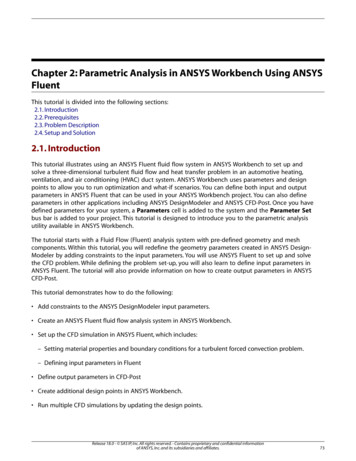
Setup and Solutionanalysis capability in ANSYS Workbench, a designer can check the performance of the system at variousdesign points.Figure 2.3: Flow Pattern for the Cooling Cycle2.4. Setup and SolutionTo help you quickly identify graphical user interface items at a glance and guide you through the stepsof setting up and running your simulation, the ANSYS Fluent Tutorial Guide uses several type styles andmini flow charts. See Typographical Conventions Used In This Manual (p. xvi) for detailed information.The following sections describe the setup and solution steps for this tutorial:2.4.1. Preparation2.4.2. Adding Constraints to ANSYS DesignModeler Parameters in ANSYS Workbench2.4.3. Setting Up the CFD Simulation in ANSYS Fluent2.4.4. Defining Input Parameters in ANSYS Fluent2.4.5. Solving2.4.6. Postprocessing and Setting the Output Parameters in ANSYS CFD-PostRelease 18.0 - SAS IP, Inc. All rights reserved. - Contains proprietary and confidential informationof ANSYS, Inc. and its subsidiaries and affiliates.77
Parametric Analysis in ANSYS Workbench Using ANSYS Fluent2.4.7. Creating Additional Design Points in ANSYS Workbench2.4.8. Postprocessing the New Design Points in CFD-Post2.4.9. Summary2.4.1. PreparationTo prepare for running this tutorial:1.Set up a working folder on the computer you will be using.2.Go to the ANSYS Customer Portal, https://support.ansys.com/training.NoteIf you do not have a login, you can request one by clicking Customer Registration onthe log in page.3.Enter the name of this tutorial into the search bar.4.Narrow the results by using the filter on the left side of the page.a.Click ANSYS Fluent under Product.b.Click 18.0 under Version.5.Select this tutorial from the list.6.Click the workbench-parameter-tutorial R180.zip link to download the input files.7.Unzip the workbench-parameter-tutorial R180.zip file to your working folder.The extracted workbench-parameter-tutorial folder contains a single archive file fluentworkbench-param.wbpz that includes all supporting input files of the starting ANSYS Workbenchproject and a folder called final project files that includes the archived final version of theproject. The final result files incorporate ANSYS Fluent and ANSYS CFD-Post settings and all alreadydefined design points (all that is required is to update the design points in the project to generate corresponding solutions).NoteANSYS Fluent tutorials are prepared using ANSYS Fluent on a Windows system. The screenshots and graphic images in the tutorials may be slightly different than the appearance onyour system, depending on the operating system or graphics card.2.4.2. Adding Constraints to ANSYS DesignModeler Parameters in ANSYSWorkbenchIn this step, you will start ANSYS Workbench, open the project file, review existing parameters, createnew parameters, and add constraints to existing ANSYS DesignModeler parameters.78Release 18.0 - SAS IP, Inc. All rights reserved. - Contains proprietary and confidential informationof ANSYS, Inc. and its subsidiaries and affiliates.
Setup and Solution1. From the Windows Start menu, select Start All Programs ANSYS 18.0 Workbench 18.0 to startANSYS Workbench.This displays the ANSYS Workbench application window, which has the Toolbox on the left and theProject Schematic to its right. Various supported applications are listed in the Toolbox, and thecomponents of the analysis system are displayed in the Project Schematic.NoteWhen you first start ANSYS Workbench, the Getting Started message window is displayed,offering assistance through the online help for using the application. You can keep thewindow open, or close it by clicking OK. If you need to access the online help at anytime, use the Help menu, or press the F1 key.2. Restore the archive of the starting ANSYS Workbench project to your working directory.File Restore Archive.The Select Archive to Restore dialog box appears.a. Browse to your working directory, select the project archive file fluent-workbench-param.wbpz,and click Open.The Save As dialog box appears.b. Browse, if necessary, to your working folder and click Save to restore the project file, fluent-workbench-param.wbpj, and a corresponding project folder, fluent-workbench-param files,for this tutorial.Now that the project archive has been restored, the project will automatically open in ANSYSWorkbench.Release 18.0 - SAS IP, Inc. All rights reserved. - Contains proprietary and confidential informationof ANSYS, Inc. and its subsidiaries and affiliates.79
Parametric Analysis in ANSYS Workbench Using ANSYS FluentFigure 2.4: The Project Loaded into ANSYS WorkbenchThe project (fluent-workbench-param.wbpj) already has a Fluent-based fluid flow analysissystem that includes the geometry and mesh, as well as some predefined parameters. You will firstexamine and edit parameters within Workbench, then later proceed to define the fluid flow modelin ANSYS Fluent.3. Open the Files view in ANSYS Workbench so you can view the files associated with the current project andare written during the session.View Files80Release 18.0 - SAS IP, Inc. All rights reserved. - Contains proprietary and confidential informationof ANSYS, Inc. and its subsidiaries and affiliates.
Setup and SolutionFigure 2.5: The Project Loaded into ANSYS Workbench Displaying Properties and Files ViewNote the types of files that have been created for this project. Also note the states of the cells for theFluid Flow (Fluent) analysis system. Since the geometry has already been defined, the status of the Geometry cell is Up-to-Date ( ). Since the mesh is not complete, the Mesh cell’s state is Refresh Required(), and since the ANSYS Fluent setup is incomplete and the simulation has yet to be performed, withno corresponding results, the state for the Setup, Solution, and Results cells is Unfulfilled (information about cell states, see the Workbench User's Guide.). For more4. Review the input parameters that have already been defined in ANSYS DesignModeler.a. Double-click the Parameter Set bus bar in the ANSYS Workbench Project Schematic to open theParameters Set tab.NoteTo return to viewing the Project Schematic, click the Project tab.Release 18.0 - SAS IP, Inc. All rights reserved. - Contains proprietary and confidential informationof ANSYS, Inc. and its subsidiaries and affiliates.81
Parametric Analysis in ANSYS Workbench Using ANSYS Fluentb. In the Outline of All Parameters view (Figure 2.6: Parameters Defined in ANSYS DesignModeler (p. 82)),review the following existing parameters: The parameter hcpos represents the valve position that controls the flow over the heat exchanger.When the valve is at an angle of 25 , it allows the flow to pass over the heat exchanger. When theangle is 90 , it completely blocks the flow towards the heat exchanger. Any value in between allowssome flow to pass over the heat exchanger giving a mixed flow condition. The parameter ftpos represents the valve position that controls flow towards the floor duct. Whenthe valve is at an angle of 20 , it blocks the flow towards the floor duct and when the valve angle is60 , it unblocks the flow. The parameter wsfpos represents the valve position that controls flow towards the windshield andthe front panel. When the valve is at an angle of 15 , it allows the entire flow to go towards thewindshield. When the angle is 90 , it completely blocks the flow towards windshield as well as thefront panel. When the angle is 175 , it allows the flow to go towards the windshield and the frontpanel.Figure 2.6: Parameters Defined in ANSYS DesignModeler5. In the Outline of All Parameters view, create three new named input parameters.a. In the row that contains New input parameter, click the parameter table cell with New name (underthe Parameter Name column) and enter input hcpos. Note the ID of the parameter that appearsin column A of the table. For the new input parameter, the parameter ID is P4. In the Value column,enter 15.b. In a similar manner, create two more parameters named input ftpos and input wsfpos. In theValue column, enter 25, and 90 for each new parameter (P5 and P6), respectively.82Release 18.0 - SAS IP, Inc. All rights reserved. - Contains proprietary and confidential informationof ANSYS, Inc. and its subsidiaries and affiliates.
Setup and SolutionFigure 2.7: New Parameters Defined in ANSYS Workbench6. Select the row (or any cell in the row) that corresponds to the hcpos parameter. In the Properties ofOutline view, change the value of the hcpos parameter in the Expression field from 90 to the expressionmin(max(25,P4),90). This puts a constraint on the value of hcpos, so that the value always remainsbetween 25 and 90 . The redefined parameter hcpos is automatically passed to ANSYS DesignModeler.Alternatively the same constraint can also be set using the expression max(25, min(P4,90)).After defining this expression, the parameter becomes a derived parameter that is dependent onthe value of the parameter input hcpos with ID P4. The derived parameters are unavailable forediting in the Outline of All Parameters view and could be redefined only in the Properties ofOutline view.ImportantWhen entering expressions, you must use the list and decimal delimiters associated withyour selected language in the Workbench regional and language settings, which correspond to the regional settings on your machine. The instructions in this tutorial assumethat your systems uses “.” as a decimal separator and “,” as a list separator.Release 18.0 - SAS IP, Inc. All rights reserved. - Contains proprietary and confidential informationof ANSYS, Inc. and its subsidiaries and affiliates.83
Parametric Analysis in ANSYS Workbench Using ANSYS FluentFigure 2.8: Constrained Parameter hcpos7. Select the row or any cell in the row that corresponds to the ftpos parameter and create a similar expressionfor ftpos: min(max(20,P5),60).84Release 18.0 - SAS IP, Inc. All rights reserved. - Contains proprietary and confidential informationof ANSYS, Inc. and its subsidiaries and affiliates.
Setup and SolutionFigure 2.9: Constrained Parameter ftpos8. Create a similar expression for wsfpos: min(max(15,P6),175).Release 18.0 - SAS IP, Inc. All rights reserved. - Contains proprietary and confidential informationof ANSYS, Inc. and its subsidiaries and affiliates.85
Parametric Analysis in ANSYS Workbench Using ANSYS FluentFigure 2.10: Constrained Parameter wsfpos9. Click the X on the right side of the Parameters Set tab to close it and return to the Project Schematic.Note the new status of the cells in the Fluid Flow (Fluent) analysis system. Since we have changedthe values of hcpos, ftpos, and wsfpos to their new expressions, the Geometry and Mesh cellsnow indicates Refresh Required ().10. Update the Geometry and Mesh cells.a. Right-click the Geometry cell and select the Update option from the context menu.b. Likewise, right-click the Mesh cell and select the Refresh option from the context menu. Once the cellis refreshed, then right-click the Mesh cell again and select the Update option from the context menu.11. Save the project in ANSYS Workbench.In the main menu, select File Save86Release 18.0 - SAS IP, Inc. All rights reserved. - Contains proprietary and confidential informationof ANSYS, Inc. and its subsidiaries and affiliates.
Setup and Solution2.4.3. Setting Up the CFD Simulation in ANSYS FluentNow that you have edited the parameters for the project, you will set up a CFD analysis using ANSYSFluent. In this step, you will start ANSYS Fluent, and begin setting up the CFD simulation.2.4.3.1. Starting ANSYS FluentIn the ANSYS Workbench Project Schematic, double-click the Setup cell in the ANSYS Fluent fluid flowanalysis system. You can also right-click the Setup cell to display the context menu where you can selectthe Edit. option.When ANSYS Fluent is first started, Fluent Launcher is displayed, allowing you to view and/or set certainANSYS Fluent start-up options.Fluent Launcher allows you to decide which version of ANSYS Fluent you will use, based on your geometryand on your processing capabilities.Figure 2.11: ANSYS Fluent Launcher1. Ensure that the proper options are enabled.ImportantNote that the Dimension setting is already filled in and cannot be changed, since ANSYSFluent automatically sets it based on the mesh or geometry for the current system.Release 18.0 - SAS IP, Inc. All rights reserved. - Contains proprietary and confidential informationof ANSYS, Inc. and its subsidiaries and affiliates.87
Parametric Analysis in ANSYS Workbench Using ANSYS Fluenta. Ensure that the Display Mesh After Reading and Workbench Color Scheme options are enabled.NoteAn option is enabled when there is a check mark in the check box, and disabled whenthe check box is empty. To change an option from disabled to enabled (or vice versa),click the check box or the text.b. Ensure that Serial is selected from the Processing Options list.NoteParallel processing offers a substantial reduction in computational time. Refer to Introduction to Using ANSYS Fluent: Fluid Flow and Heat Transfer in a Mixing Elbow (p. 121)in this manual and the Fluent User's Guide for further information about using theparallel processing capabilities of ANSYS Fluent.c. Ensure that the Double Precision option is disabled.NoteFluent will retain your preferences for future sessions.2. Click OK to launch ANSYS Fluent.88Release 18.0 - SAS IP, Inc. All rights reserved. - Contains proprietary and confidential informationof ANSYS, Inc. and its subsidiaries and affiliates.
Setup and SolutionFigure 2.12: The ANSYS Fluent Application2.4.3.2. Setting Up Physics1. In the Solver group of the Setting Up Physics ribbon tab, retain the default selection of the steady pressurebased solver.Setting Up Physics Solver2. Set up your models for the CFD simulation using the Models group of the Setting Up Physics ribbon tab.a. Enable heat transfer by activating the energy equation.Release 18.0 - SAS IP, Inc. All rights reserved. - Contains proprietary and confidential informationof ANSYS, Inc. and its subsidiaries and affiliates.89
Parametric Analysis in ANSYS Workbench Using ANSYS FluentIn the Setting Up Physics ribbon tab, select Energy (Models group).Setting Up Physics Models Energyb. Enable the -turbulence model.Setting Up Physics Models Viscous.i.Select k-epsilon (2 eqn) from the Model group box.ii. Select Enhanced Wall Treatment from the Near-Wall Treatment group box.90Release 18.0 - SAS IP, Inc. All rights reserved. - Contains proprietary and confidential informationof ANSYS, Inc. and its subsidiaries and affiliates.
Setup and SolutionThe default Standard Wall Functions are generally applicable when the cell layer adjacent to thewall has a y larger than 30. In contrast, the Enhanced Wall Treatment option provides consistentsolutions for all y values. Enhanced Wall Treatment is recommended when using the k-epsilonmodel for general single-phase fluid flow problems. For more information about Near WallTreatments in the k-epsilon model refer to the Fluent User's Guide.iii. Click OK to retain the other default settings, enable the model, and close the Viscous Model dialogbox.Note that the Viscous. label in the ribbon is displayed in blue to indicate that the Viscousmodel is enabled.3. Define a heat source cell zone condition for the evaporator volume.Setting Up Physics Zones Cell ZonesNoteAll cell zones defined in your simulation are listed in the Cell Zone Conditions task pageand under the Setup/Cell Zone Conditions tree branch.a. In the Cell Zone Conditions task page, under the Zone list, select fluid-evaporator and click Edit.to open the Fluid dialog box.b. In the Fluid dialog box, enable Source Terms.c. In the Source Terms tab, click the Edit. button next to Energy.Release 18.0 - SAS IP, Inc. All rights reserved. - Contains proprietary and confidential informationof ANSYS, Inc. and its subsidiaries and affiliates.91
Parametric Analysis in ANSYS Workbench Using ANSYS Fluentd. In the Energy sources dialog box, change the Number of Energy sources to 1.e. For the new energy source, select constant from the drop-down list, and enter -787401.6 W/m3 —based on the evaporator load (200 W) divided by the evaporator volume (0.000254 m3) that was computed earlier.f.Click OK to close the Energy Source dialog box.g. Click OK to close the Fluid dialog box.2.4.4. Defining Input Parameters in ANSYS FluentYou have now started setting up the CFD analysis using ANSYS Fluent. In this step, you will defineboundary conditions and input parameters for the velocity inlet.1. Define an input parameter called in velocity for the velocity at the inlet boundary.a. In the Setting Up Physics tab, click Boundaries (Zones group).Setting Up Physics Zones BoundariesThis opens the Boundary Conditions task page.NoteAll boundaries defined in the case are also displayed under the Setup/BoundaryConditions tree branch.b. In the Boundary Conditions task page, click the Toggle Tree View button (in the upper right corner),and under the Group By category, select Zone Type. This displays boundary zones grouped by zonetype.c. Under the Inlet zone type, double-click inlet-air.92Release 18.0 - SAS IP, Inc. All rights reserved. - Contains proprietary and confidential informationof ANSYS, Inc. and its subsidiaries and affiliates.
Setup and Solutiond. In the Velocity Inlet dialog box, from the Velocity Magnitude drop-down list, select New InputParameter.This displays the Input Parameter Properties dialog box.e. Enter in velocity for the Name, and enter 0.5 m/s for the Current Value.f.Click OK to close the Input Parameter Properties dialog box.g. Under the Turbulence group box, from the Specification Method drop-down list, select Intensityand Hydraulic Diameter.h. Retain the value of 5for Turbulent Intensity.Release 18.0 - SAS IP, Inc. All rights reserved. - Contains proprietary and confidential informationof ANSYS, Inc. and its subsidiaries and affiliates.93
Parametric Analysis in ANSYS Workbench Using ANSYS Fluenti.Enter 0.061 for Hydraulic Diameter (m).2. Define an input parameter called in temp for the temperature at the inlet boundary.a. In the Thermal tab of the Velocity Inlet dialog box, select New Input Parameter. from theTemperature drop-down list.b. Enter in temp for the Name and enter 310 K for the Current Value in the Input ParameterProperties dialog box.c. Click OK to close the Input Parameter Properties dialog box.d. Click OK to close the Velocity Inlet dialog box.3. Review all of the input parameters that you have defined in ANSYS Fluent under the Parameters & Customization/Parameters tree branch.Parameters & Customization Parameters Input ParametersFigure 2.13: The Input Parameters Sub-Branch in ANSYS Fluent94Release 18.0 - SAS IP, Inc. All rights reserved. - Contains proprietary and confidential informationof ANSYS, Inc. and its subsidiaries and affiliates.
Setup and SolutionThese parameters are passed to ANSYS Fluent component system in ANSYS Workbench and areavailable for editing in ANSYS Workbench (see Figure 2.14: The Parameters View in ANSYS Workbench (p. 95)).Figure 2.14: The Parameters View in ANSYS Workbench4. Set the turbulence parameters for backflow at the front outlets and foot outlets.a. In the Boundary Conditions task page, type outlet in the Zone filter text entry field. Note that asyou type, the names of the boundary zones beginning with the characters you entered appear in theboundary condition zone list.Note The search string can include wildcards. For example, entering *let* will display all zonenames containing let, such as inlet and outlet. To display all zones again, click the red X icon in the Zone filter.b. Double-click outlet-front-mid.Release 18.0 - SAS IP, Inc. All rights reserved. - Contains proprietary and confidential informationof ANSYS, Inc. and its subsidiaries and affiliates.95
Parametric Analysis in ANSYS Workbench Using ANSYS Fluentc. In the Pressure Outlet dialog box, under the Turbulence group box, select Intensity and HydraulicDiameter from the Specification Method drop-down list.d. Retain the value of 5 for Backflow Turbulent Intensity (%).e. Enter 0.044 for Backflow Hydraulic Diameter (m).These values will only be used if reversed flow occurs at the outlets. It is a good idea to set reasonablevalues to prevent adverse convergence behavior if backflow occurs during the calculation.f.Click OK to close the Pressure Outlet dialog box.g. Copy the boundary conditions from outlet-front-mid to the other front outlet.Setup Boundary Conditions outlet-front-mid96Copy.Release 18.0 - SAS IP, Inc. All rights reserved. - Contains proprietary and confidential informationof ANSYS, Inc. and its subsidiaries and affiliates.
Setup and Solutioni.Confirm that outlet-front-mid is selected in the From Boundary Zone selection list.ii. Select outlet-front-side-left in the To Boundary Zones selection list.iii. Click Copy to copy the boundary conditions.Fluent will display a dialog box asking you to confirm that you want to copy the boundary conditions.iv. Click OK to confirm.v. Close the Copy Conditions dialog box.h. In a similar manner, set the backflow turbulence conditions for outlet-foot-left using the values in thefollowing table:ParameterValueSpecification MethodIntensity and Hydraulic DiameterBackflow Turbulent Intensity (%)5Backflow Hydraulic Diameter (m)0.0522.4.5. SolvingIn the steps that follow, you will set up and run the calculation using the Solving ribbon tab.NoteYou can also use the task pages listed under the Solution branch in the tree to performsolution-related activities.1. Set the Solution Methods.Solving Solution Methods.Release 18.0 - SAS IP, Inc. All rights reserved. - Contains proprietary and confidential informationof ANSYS, Inc. and its subsidiaries and affiliates.97
Parametric Analysis in ANSYS Workbench Using ANSYS FluentThis will open the Solution Methods task page.a. From the Scheme drop-down list, select Coupled.The pressure-based coupled solver is the recommended choice for general fluid flow simulations.b. In the Spatial Discretization group box, configure the following t Order UpwindEnergyFirst Order UpwindRelease 18.0 - SAS IP, Inc. All rights reserved. - Contains proprietary and confidential informationof ANSYS, Inc. and its subsidiaries and affiliates.
Setup and SolutionThis tutorial is primarily intended to demonstrate the use of parameterization and design pointswhen running Fluent from Workbench. Therefore, you will run a simplified analysis using firstorder discretization, which will yield faster convergence. These settings were chosen to speed upsolution time for this tutorial. Usually, for cases like this, we would recommend higher orderdiscretization settings to be set for all flow equations to ensure improved results accuracy.2. Initialize the flow field using the Initialization group of the Solving ribbon tab.Solving Initializationa. Retain the default selection of Hybrid Initialization.b. Click the Initialize button.3. Run the simulation in ANSYS Fluent from the Run Calculation group of the Solving tab.Solving Run Calculationa. For Number of Iterations, enter 1000.b. Click the Calculate button.The solution converges within approximately 55 iterations.Throughout the calculat
analysis capability in ANSYS Workbench, a designer can check the performance of the system at various design points. Figure 2.3: Flow Pattern for the Cooling Cycle 2.4. Setup and Solution To help