Transcription
Summer Institute in Statistical GeneticsModule 20: Advanced R Programmingfor bioinformaticsThomas LumleyKen RiceUniversities of Washington and AucklandSeattle, June 2011
Introduction: Course Aims Programming with R– Efficient coding– Code that other people can use Using R for sophisticated analyses– Some useful tools for large-scale problems– Making R play nicely with others– Knowing where to look when you need more0.1
Introduction: About Prof Lumley Associate Prof, UW Biostat R Core developer Genetic/Genomic research inCardiovascular Epidemiology Sings bass0.2
Introduction: About Prof Rice Assistant Prof, UW Biostat Not an authoR, but a useR (anda teacheR) Genetic/Genomic research inCardiovascular Epidemiology Sings bass. and you?(who are you, what area of genomics, what are you looking forfrom the course)0.3
Introduction: Course structure10 sessions over 2.5 days Day 1; Programming in R, Graphics Day 2; Objects, packages, XML Day 3; C code, large datasetsDownload everything from v0.4
Introduction: Session structureWe will alternate teaching (questions welcome) and hands-onexercisesFor some topics, within a single 90 minute session; 45 mins teaching (Questions welcome! Please interrupt!) 30 mins hands-on 15 mins summary, discussionFor other topics, we’ll separate sessions (90 mins) and hands-onexercises (90 mins)0.5
1. Introduction to R:First stepsKen RiceThomas LumleyUniversities of Washington and AucklandSeattle, June 20111.0
Important pre-takeoff announcement:We are assuming you know; How to use R from the command line, and how to write anduse script files (and spot e.g. missing commas and }’s ) How to manipulate basic data structures in R; in particularvectors and data frames How to write functions What NA means, and that 42 NA NA Enough programming (in R or elsewhere) to recognize loops,and manage files external to your R session How to look up help filesOf course, familiarity with (non-advanced) statistical & geneticconcepts will also help1.1
Programmers: what is R? R is a free implementation of a dialect of the S language, theinteractive statistics and graphics environment developed atBell Labs. R/S are probably the most widely used software for researchin statistical methodology and in genomics, and is popular infinancial modelling and medical statistics. John Chambers won the 1999 ACM Software Systems awardfor S, which will forever alter the way people analyze,visualize, and manipulate data. Ross Ihaka won the Royal Society of New Zealand’s 2008Pickering Medal, recognizing excellence and innovation in thepractical application of technology for the creation of R.1.2
Programmers: a little prehistoryThe design of R is largely based on S version 3, which predatesJava, Python, JavaScript, Linux, MacOS X, and usable versionsof Windows.Much of the design was fixed in S version 2, which predatesC , Perl, the ANSI C standard, the IBM PC, the GNU project,and Miami Vice.The basic graphics system is older than Space Invaders.Yes, some things would be done differently today.1.3
SimulationThis really is how calculations and simulation studies were done!Simulations have always been part of statistical research.1.4
Simulations: a simple example?Here’s a simple problem, for which we can work out the exactanswer;0.60.0Exp(1) looks like this (right)any guesses?0.20.4densityIf you had, say, 51 survival timesto analyze, from a distributionof times not unlike Exp(1),these are sane questions.0.81.0For samples of i.i.d Exp(1) data with n 51.What is the mean value of the sample median?What is the mean value of the median-squared?012345x1.5
Simulations: a simple example?.guessing these would require a lot of luck;EY EY 2 657749001278815379823900480000 They are 0.70286, 0.51380, to 5 d.p. They are about 2/3 and 1/2 3–4 significant figures is probably enough for most practicalpurposes. Being able compute more accurately is re-assuring In the ‘post-genome’ era, being able to compute quickly isimportant (again)1.6
Simulations: a simple example?Brute force provides perfectly acceptable answers; the replicate()function replicates evaluation of an expression bigB - bazillion - 10000 set.seed(4) # a specific "start" value many.medians - replicate(bigB, { median(rexp(51)) } ) round( mean(many.medians), 3)[1] 0.702 round( mean(many.medians 2), 3)[1] 0.513The ‘right’ answers averages over an infinite number of replicatsions. bigB 10,000 here, which .This calculation takes 2 seconds, on my desktop1.7
Simulations: a simple example?Our simulations get us very close to the true distribution of themedian;1.00.0Density2.0Histogram of many.medians0.00.51.01.52.0medianHaving done the ‘hard work’ of simulation, we can also computeskewness, kurtosis, quantiles, etc – all for ‘free’. This techniqueis very powerful – and often under-rated by statisticians.1.8
Simulations: a simple example?Here are some other statistical concepts, interpreted in the sameway; [If] we simulated data, a bazillion times (B ).” .and applied our procedure to each dataset – and recordedthe output Does our estimate usually get close? [consistency]How close does our estimate typically get? [bias]How variable is our estimate? [standard error, efficiency]How often does our interval cover the truth? [coverage]How often does our test make a Type I/Type II error?[size/power]1.9
Effective codingWe need to be able to program simulations effectively. A gooddefault for any simulation study follows this ‘pseudo-code’;do.one - function(n, beta, f){. commands to do one analysis. last command spits out what you want}many.sim - replicate(bigB, do.one(my.n, my.beta, my.f)). commands to work out observed coverage, bias, etcOnce this works, wrap it inside further loops, e.g.n.vals - c(10, 20, 30, 40, 50, 1000)coverage.vals - sapply(n.vals, function(n){. commands to do the replication, with my.n n})At each stage, you must first write a function, then check it.This requires a bit of sanity-checking (i.e. trying it where youknow at least roughly what should happen) and debugging.1.10
Effective codingThe use of sapply() (and apply(), lapply() ) can be unfamiliar– many programmers have used for() loops elsewhere. R doeshave for() loops (see ?Control) but; ‘Growing’ the dataset is a terrible idea;mydata - cbind(mydata, rnorm(1000, mean i)) # nooooo!Always set up blank output first, then ‘fill it in’ Use of replicate(), apply() etc means slightly faster interpretation of code than for() – but not by much. for() loopsare not intrinsically evil for() requires more typing than replicate() etc, and is oftenmore work to edit Using functions makes your ultimate R package easier toproduce. right?1.11
DebuggingA ‘handy’ hint from the Apple Corporation;1.12
DebuggingBeyond the level of spotting missed commas and mis-matchingparentheses, debugging is difficult.We’ll discuss use of traceback() and recover(), which can help; # a trite example of traceback() f1 - function(x){ print(x); f2(x) } f2 - function(x){ x i.dont.exist } f1(10) # gives this strange error;[1] 10Error in f2(x) : object ’i.dont.exist’ not found traceback()2: f2(x)1: f1(10)The error occurred inside the execution of f2()1.13
DebuggingIf the error’s not obvious, try using recover();options(error recover) # enter c to closeset.seed(4)replicate(1000, {y - rnorm(10)x - rbinom(10, 1, 0.5)lm1 - lm(y x) # regress Y on Xc(coef(lm1)[2], vcov(lm1, "HC0")[2,2]) # terms of interest})#turn it off! turn it off!options(error NULL)Use ls() to list local objects; the highest frame number is a goodplace to start1.14
Debuggingtrace() adds instrumentation to a function trace(rnorm) prints a message when rnorm is started/ended trace(rnorm, recover) calls the debugger when rnorm() isentered. trace(lm, quote(if(all(mf x 1)) recover()), at 12) calls thedebugger if mf x is all 1s at line 12 of lm()Use untrace(rnorm) to remove tracing from rnorm()1.15
ExceptionsWhile you might never see them in practice (due to datacleaning) in simulation studies your replications may produce‘pathological’ data, e.g. all X are identical, or all minor allelecarriers smoke. If your regressions estimate differences per allelecopy, adjusting for smoking, it should complain.If this is just too tedious (and rare) to bother fixing, you can usetryCatch();one.glm - function(outcome, x){tryCatch({model - glm(outcome x, family binomial())coef(summary(model))[2,]},error function(e) rep(NA, 4))}. but check your simulation output’s rates of NA-ness.better to pre-empt these problems – but this is not easyIt’s1.16
TimingPremature optimization is the root of all evilDonald KnuthIf you already have the capacity to generate reasonably accurateresults within a sane time limit, optimizing code is a waste ofeffortIf you need to do things an order of magnitude faster, or useyour code again (repeatedly) then optimizing your code may beworthwhileTo optimize, you need to know; What’s the bottleneck? How much faster can I make that step?1.17
TimingObvious bottleneck/easy solution;1.18
Timing.What’s the bottleneck?Experienced useRs may be able to ‘eyeball’ this from code;measurement is an easier and more reliable approach (!)To find out how long operations are taking; proc.time() returns the current time. Save it before a taskand subtract from the value after a task. system.time() times the evaluation of a given expression R has a profiler; this records which functions are being run,many times per second. Rprof(filename) turns on the profiler,Rprof(NULL) turns it off. summaryRprof(filename) reports howmuch time was spent in each function.Remember: A 1000-fold speedup in a function used 10% of thetime is less helpful than a 2-fold speedup in a function used50% of the time.1.19
TimingA small example of this in action;# what is taking all the time?Rprof("deleteme.txt")many.sim - replicate(1000, {y - rnorm(10)x - rbinom(10, 1, 0.5)if( all(x 0) all(x 1)) return(c(NA,NA))lm1 - lm(y x)c(coef(lm1)[2], vcov(lm1)[2,2])})Rprof(NULL) # turn it off! turn it off!summaryRprof("deleteme.txt")1.20
Timing.How much faster can I make that step?Some simple tips; Pre-process/clean your data before analysis; e.g. sum(x)/length(x)doesn’t error-check like mean(x) Similarly, use glm.fit not glm – use matrix calculations inplace of lm() Use vectorized operations, where possible Store data as matrices, not data frames Delete objects you are finished with1.21
TimingMore advanced methods; Write small but important pieces of code in C, and callthese from R Run multiple batches. Store your commands in one scriptfile (which you should do anyway) and call it with e.g.R CMD BATCH myscript.R myconsoleoutput.txt &. and finally assemble all the (saved) resultsThe second option applies when there is no available speedup; ifyour R session is mostly waiting for C to do matrix work, writingthe whole thing in C offers no important benefit1.22
More advanced: short cuts to CFor a limited number of jobs, it may be worth getting R to senda (large) number of generated datasets to C simultaneously. For example, instead of looping over datasets with n 20outcomes Y and n 20 covariates X , generate B 20matrices Y and X; using rowSums(X), rowSums(X*Y) etc toconstruct β̂ avoids replicate() or similar For large n or large B one can quickly run out of memory This is a massive pain! I have only used it productively forone real job – doing 2.5 million cookie-cutter meta-analyses Less of a pain is cor(large.matrix) – for all pairwise correlations of columns of large.matrix, where all the looping isdone in CFor complex methods, this approach will not help1.23
Bonus tracks: how big?Q. What’s the ‘Monte Carlo’ error in my estimates?One quick-and-dirty measure of uncertainty is given by theseintervals;many.thetahat - replicate(bigB, {.calculate an estimate.} )lm1 - lm(many.thetahat 1)confint.default(lm1)For binary outcomes, (i.e. when you want coverage, size, power)z - replicate(bigB, {. calculate theta.hat/est.std.err .})mean( z 2 1.96 2 ) # how many give p 0.05?lm2 - lm( I(z 2 1.96 2) 1 )confint.default(lm2)For GWAS-style levels of e.g. 5 10 8, simulations with e.g.B 1010 may be needed; efficient coding of them can savemany days of processor time.1.24
Module 20: Advanced R Programming for bioinformatics Thomas Lumley Ken Rice Universities of Washington and Auckland Seattle, June 2011. Introduction: Course Aims Programming with R { E cient coding { Code that other people can use Using R for sophistica