Transcription
MATHEMATICS OF MEDICAL IMAGINGINVERTING THE RADON TRANSFORMKAILEY BOLLESAbstract. Computed Tomography (CT) and other radial imaging techniquesare vital to the practice of modern medicine, allowing non-invasive examinationof the inner workings of the human body. However, raw CT data must betransformed in order to become diagnostically relevant. This project examinesraw CT data, modeled by the Radon transform, and methods of inversion viaunfiltered backprojection, Fourier transforms, and filtered backprojection (theinverse Radon transform). We demonstrate this process through examples of“raw data” and inversion, with a focus on the influence of discrete data setsof different sizes on inversion quality.1. IntroductionThe study of medical imaging has led to techniques vital to the practice ofmedicine, such as x-ray imaging, computed tomography (CT) scans, magnetic resonance imaging, and a variety of other radiological imaging techniques. Such techniques allow the examination of the internal condition of the body without theuse of invasive surgical procedures. Tomography, or slice imaging, represents asubset of these techniques, notably x-ray imaging and CT scans, used to translatetwo-dimensional external measurements into a reconstruction of three-dimensionalinternal structure. This investigation will focus on CT scans, although the mathematics of CT scans are very similar to those used in other types of medical imaging.CT scans are of particular practical interest because they are useful in diagnosingskeletal damage, cancers, and vascular diseases. They can also be used to guidesurgery, biopsy, and radiation therapy in real time.Many of the discussions found in this paper are adapted from Charles Epstein’s Introduction to the Mathematics of Medical Imaging [1], Peter O’Neil’s Advanced Engineering Mathematics [2], and Yves Nievergelt’s Elementary Inversion ofRadon’s Transform [3]. These publications, particularly [1], also represent valuablesources for those desiring further information on these topics.1.1. X-Ray Imaging. X-ray imaging relies on the principle that an object willabsorb or scatter x-rays of a particular energy in a manner dependent on its composition, quantified by the attenuation coefficient µ. The attenuation coefficient µof a substance is a function in R3 dependent on a variety of factors, but primarilyreflective of the electron density of that substance. Therefore, denser substancesand substances containing elements with many electrons will have higher attenuation coefficients. This helps explain why bone, which contains high percentages ofcalcium (20 electrons), potassium (19 electrons), phosphorous (15 electrons), andmagnesium (12 electrons), has a much higher attenuation coefficient than soft tissue, which is made up primarily of carbon (6 electrons), nitrogen (7 electrons), and1
2KAILEY BOLLESFigure 1. A 2D diagram of a CT scanner. The CT scanner ismade up of a point-source emitter and film that rotate aroundan object of interest, imaging the object in 2D slices and thencompiling these slices into a 3D rendering of the object. Imagefrom [1].oxygen (8 electrons) [1]. Air is considered to have an attenuation coefficient of zerofor simplicity of calculation, so the attenuation coefficient disappears outside thebody.In practice, Hounsfield units–attenuation coefficients normalized to the attenuation coefficient of water–are used in favor of attenuation coefficients. This is dueto the fact that these units are suited to the examination of organisms primarilycomposed of water, e.g., humans. The Hounsfield unit of a tissue is defined byHtissue µtissue µwater 1000.µwater(from [1])Although this examination will focus on the mathematics of the attenuationcoefficient itself, it is important to consider the practical ramifications representedby the Hounsfield unit representation of particular tissues. The typical clinicalrange of a CT scan, between air and bone, is approximately 2000 H [1]. Soft tissue,the primary target of clinical investigation, represents a very small fraction of thisrange, meaning that CT scans must be extremely sensitive in order to be clinicallyuseful.1.2. CT Scanning. Computed tomography scanning is essentially an extrapolation of the concept of an x-ray. Instead of taking a single x-ray from a singleperspective, a CT scan rotates a point source of x-rays around a body to be imaged. This exposes film on the opposite side of the object. By making calculationsfrom the level of exposure (density) of the film, one can determine line integrals ofthe attenuation coefficient µ through the object. Taking the calculations from afull rotation, it is possible to reconstruct the 2D slice of the object. Compilation ofmultiple slices allows for 3D reconstruction of the object.
MATHEMATICS OF MEDICAL IMAGING3Essentially, the mathematics of CT scanning involves two problems. In theforward problem, we model the data obtained from real-world CT scans using theRadon transform. The Radon Transform allows us to create “film images” of objectsthat are very similar to those actually occurring in x-rays or CT scans. The inverseproblem allows us to convert Radon transforms back into attenuation coefficientsusing the inverse Radon transform–to reconstruct the body from a CT scan.1.3. Thesis Objectives. This thesis addresses both the forward and inverse problems of medical imaging and the Radon transform. Section 2 examines the parametrization and definition of the Radon transform, showing how we obtain the “mock CT”transform data by applying the Radon transform to known functions. A simple inversion technique called unfiltered backprojection–and its drawbacks–are examinedin Section 3. Section 4 begins a discussion of another common data transform calledthe Fourier transform, which is linked to the Radon transform by the Central SliceTheorem discussed in Section 5. Sections 6 and 7 address methods of applying theFourier transform to discrete, real-world data–the discrete Fourier transform andthe sampled Fourier transform, respectively. An inversion formula for the Radontransform is presented and proved with calculus in Section 8. Section 9 presentsa simple “body” as an example of moving through the process of Radon transform/CT data reconstruction and shows the effect of different levels of discretedata on reconstructions. The paper concludes and presents possibilities for furtherexploration in Section 10.2. The Radon TransformIn order to work in the circular geometry of CT scans, it is helpful to parametrizelines ax by c in R2 to a set of oriented lines with radial parameters t,θ in R S 1(see figure 2). In medical imaging, these lines are representative of the trajectoriesof x-ray beams entering a body. Consider the general line in R2(1)ax by c,where a, b, and c are constants. We then havebcax y .2222 ba ba b2 The first two coefficients, a2a b2 , a2b b2 , define a point on the unit circle. Letθ be the angle corresponding to that point on the unit circle, so aθ cos 1 .a2 b2 a2Then cos θ a2a b2 and sin θ a2b b2 . This parametrization has an intrinsicrepetitive quality; the angle θ can only take on values of [0, π) before repeatingpreviously described lines. Let t be the distance from the origin to the line ax by c along the angle θ. Then the line can also be described as the set of solutions (x, y)to the inner productt h(x, y), (cos θ, sin θ)i h(x, y), ωi.Therefore, t is equal to the right side of equation (1). Notice that our definitionsof t and θ also give us a point on the line, (t cos θ, t sin θ), where a line at angle θ
4KAILEY BOLLESFigure 2. The parametrization of lines ax by c to lines t,θ in R2 .intersects ax by c. This intersection is a right angle, because while the slope ofthe line ax by c is ab , the tangent of θ issin θb .cos θaLet the vector ω hcos θ, sin θi, perpendicular to the line ax by c, and let thevector ω̂ h sin θ, cos θi be parallel to this line. We can therefore create a vectorequation in terms of t and θ for the line,tan θ t,θ tω sω̂ ht cos θ, t sin θi sh sin θ, cos θi,where s R. This line is the same as the line ax by c, but the parametrizationis in terms of an affine parameter t and the angular parameter θ, making it easierto determine a set of lines emanating from or passing through a single point.
MATHEMATICS OF MEDICAL IMAGING5Figure 3. The piecewise-defined function g.Definition 2.1. Let f be some function in R2 , parametrized over the lines t,θ .The Radon transform Rf (t, θ) is defined asZZ Z Rf (t, θ) f ds f (tω sω̂)ds f (t cos θ s sin θ, t sin θ s cos θ)ds. t,θ This definition describes the Radon transform for an angle θ. These discrete-θRadon transforms can be combined, taking the integral of a function f over all lines t,θ in R S 1 . For our purposes, it accurately models the data acquired from takingcross-sectional scans of an object from a large set of angles, as in CT scanning, andits inverse can be used to reconstruct an object from CT data.To illustrate this process, consider the following simple example function 1 (x 1)2 y 2 11 (x 2)2 y 2 41g(x, y) 0 everywhere else,shown in figure 3.Taking the Radon transform R for discrete values of θ, we acquire a set of “lineprofiles” of the intensity of g at an angle perpendicular to the angle θ (see figure 4).These profiles are perpendicular due our initial parametrization, in which the lineof interest t,θ is perpendicular to the vector hcos θ, sin θi.The Radon transform R of the function g, plotted over all values of t and θ, canbe seen in figure 5. This image represents a collection of all of the possible discreteRadon transforms (such as those shown in figure 4), where the axes represent the tand θ values and the color brightness represents the intensity/density of the function(the vertical scale of figure 4) at a particular point.3. Unfiltered BackprojectionThe Radon transform is helpful to tomography applications such as CT becauseit can model the data originally obtained from such scans. However, such data isnot immediately applicable to diagnostic applications because it does not directly
6KAILEY BOLLESFigure 4. Radon transform R(g) of the piecewise-defined function g at the angles θ 0 (upper left), θ π3 (upper right), θ π2(lower left), and θ π (lower right). Note that in this parametrization, the angle θ is perpendicular to the angle of the line passingthrough the object. Image created using Maple.resemble the object being imaged. A method of recreating the original image (inthe case of the Radon transform itself, the original function) with a high degree ofspecificity and veracity is therefore required in order to apply tomographic technologies in the real world. Perfect reconstruction via abstract inversion is possiblefor continuous data (i.e., functions) but the finite (discrete) data available in thereal world allows for only estimated reconstructions. Thus most work for CT andother real-world applications focuses on improving these estimates.An initially appealing method is unfiltered backprojection, which takes the average values of the function along each line and “smears” or projects them backover the line in order to create an image.
MATHEMATICS OF MEDICAL IMAGING7Figure 5. The Radon transform of the function g over all valuesof t and θ. The brightness of the image represents the “density”of the function g at a particular point. Image created using MATLAB.Definition 3.1 (from [1]). Let f be some function in R2 , parametrized over thelines t,θ . The unfiltered backprojection B [f (t, θ)] is defined asZ 2π1B [f (t, θ)] Rf (t, θ)dθ.2π 0Unfiltered backprojection is a simple and logical computation, but not a faithfulrepresentation of f , as can be observed in the graphs of the two-circle example function g and its unfiltered backprojection in figure 6. The unfiltered backprojectionretains the basic characteristics of g, but it loses contrast and introduces imaging artifacts (i.e., radial blur). This is not particularly problematic for a simple,high contrast image like the example function g. However, in medical applicationswhere the areas of interest are likely soft tissues with highly similar attenuation coefficients, loss of contrast and introduction of imaging artifacts would likely renderan image completely useless. Therefore unfiltered backprojection is not a viable
8KAILEY BOLLESFigure 6. The example function g (left) and its unfiltered backprojection (right). Backprojection created using MATLAB.solution to the problem of inverting the Radon transform for medical imaging applications.As unfiltered backprojection’s lack of specificity renders it unusable for medicalimaging applications, we must examine other methods for inverting the Radontransform. The Radon transform is closely related to the Fourier transform, anextensively studied method whose inverse is well-described, by the Central SliceTheorem. We will introduce the Fourier transform before exploring this relationshipfurther. Derivations and notation for this section will closely follow [2].4. Fourier Transform DerivationR Suppose a function f is absolutely integrable, that is, that f (x) dx converges and f is piecewise smooth on every interval [ L, L]. Then the Fourier seriesfor f on this arbitrary interval is!Z LZ nπυ nπx X11 LF S[f (υ)] f (υ)dυ f (υ) cosdυ cos 2L LL LLLn 1!Z nπυ nπx X1 L f (υ) sindυ sin.L LLLn 1πTo simplify these equations, let ωn nπL and ωn ωn 1 L ω, so thatω becomes angular frequency and conveniently absorbs the angular terms of theFourier series. Then the Fourier series of f becomes!!Z LZ L 1X1f (υ)dυ ω f (υ) cos(ωn υ)dυ cos(ωn x) ω F S[f (υ)] 2ππ n 1 L L!Z L 1X(2) f (υ) sin(ωn υ)dυ sin(ωn x) ω.π n 1 LIn order to get an approximation for the whole real line, let us examine the Fourierseries of f as L approaches infinity. Letting L approach infinity causes ω to
MATHEMATICS OF MEDICAL IMAGING9approach zero. The first component of equation (2) will therefore also approachzero, that is,!Z L1as ω 0,f (υ)dυ ω 0,2π Lbecause we assumed that f was absolutely convergent. Therefore, equation (2)approaches Z Z Z 1 f (υ) sin(ωυ)dυ sin(ωx) dω,f (υ) cos(ωυ)dυ cos(ωx) π 0 as L approaches infinity. This is the Fourier integral of f on the real line. If f iscontinuous at x, this integral converges to f (x). If there is a jump discontinuity inf , the integral will return the average of the values of the function lim f (x) andx alim f (x) on either side of the jump. Using trigonometric identities, the Fourierx a integral can also be expressed asZ Z1 F I[f (υ)] f (υ) cos(ω(υ x))dυdω.π 0 The complex form of the cosine function in this case is 1 iω(υ x)cos(ω(υ x)) e e iω(υ x) .2If we insert this complex form into the Fourier integral, we eventually find thatZ 1F I[f (υ)] Ceiωx dω,2π R where C f (t)e iωt dt. This is the complex Fourier integral of f , and itscoefficient C is the Fourier transform of f , also written as fˆ(ω).Definition 4.1. Let f (x) be an absolutely integrable function with frequency ω.Then the Fourier transform fˆ(ω) (also written as F[f (x)](ω)) is defined asZ ˆf (ω) f (x)e iωx dx. Definition 4.2. Let F (ω) be an absolutely integrable function. Then the inverseFourier transform fˇ(x) (also written as F 1 [F (ω)](x)) is defined asZ 1fˆ(ω)eiωx dω.fˇ(x) F 1 [F (ω)](x) 2π Consider the case where F (ω) is an absolutely integrable Fourier transform ofa function that is also absolutely integrable. If both functions satisfy estimates ofthe formQ F (ω) for aδ 0,(1 ω )1 δP f (x) for an 0,(1 x )1 where P and Q are upper limits on both the functions and their derivatives, thenthe inverse Fourier transform of the Fourier transform F (ω) of f (x) will equal theoriginal function f (x),ˇfˆ(x) F 1 [F[f (x)](ω)] (x) f (x).
10KAILEY BOLLESIn order to work in two-dimensional CT geometry, it is helpful to include anextension of the Fourier transform into two dimensions. Its derivation is similar, butconsiders two angular frequencies r and ω, operating in the two different directionsof the plane.Definition 4.3. Let f (x, y) be an absolutely integrable function. Then the twodimensional Fourier transform fˆ(r, ω) is defined asZ Z f (x, y)e irω·hx,yi dxdy.fˆ(r, ω) 5. Central Slice TheoremHaving defined both the Radon transform and the Fourier transform, we cannow explore the Central Slice Theorem, which connects the two transforms. Thisdiscussion closely parallels that found in [1].Theorem 5.1. Let the natural domain of R be defined as those functions whichare piecewise continuous and satisfy an estimate of the form f (ξ) Q(1 ξ )1 for an 0,where ξ tω sω̂ and Q is an upper limit on both the Radon transform and itsderivative. Let f be an absolutely integrable function in this domain. For any realnumber r and unit vector ω hcos θ, sin θi, we have the identityZ Rf (t, θ)e itr dt fˆ(r, ω). Proof. Begin by substituting the definition of R into the first statement of theidentity to obtainZ Z Z Rf (t, θ)e itr dt f (tω sω̂)e itr dsdt, where ω̂ h sin θ, cos θi, the vector perpendicular to ω. Performing the change ofvariables ξ tω sω̂ we findZ Z Zf (tω sω̂)e itr dsdt f (ξ)e itr dξ R2Z Z f (x, y)e irω·hx,yi dxdy fˆ(r, ω). Therefore, the two-dimensional Fourier transform fˆ(r, ω) is the one-dimensionalFourier transform of Rf (t, θ).In order to better understand how the two-dimensional Fourier transform fˆ(r, ω)is equivalent to the one-dimensional Fourier transform of Rf (t, θ), let us consideran example. Let θ 0 so that ω (cos θ, sin θ) becomes the unit vector (1,0) and
MATHEMATICS OF MEDICAL IMAGING11ω̂ is the unit vector (0,1), perpendicular to ω. The Radon transform Rf (t, θ) isthenZ Rf (t, θ) f (tω sω̂) ds Z f (t · (1, 0) s · (0, 1)) ds Z f (t, s) ds. Then the Fourier transform of Rf (t, θ) isZ Z ZRf (t, θ)e irt dt f (t, s)e irt dsdt, where r is a constant. Since the inner product hrω, (t, s)i rt, the last statementis the definition of the two-dimensional Fourier transform fˆ(r, ω).6. Discrete Fourier TransformIn medical imaging, we are not working with continuous inputs (e.g., functions orinfinite data sets) but with discrete ones (e.g., real-world, finite data). Therefore wecannot directly apply the Central Slice Theorem and Fourier transform, because itapplies to continuous data. We need a method for modeling the Fourier transformof discrete data: the discrete Fourier transform. 1Definition 6.1 (from [2]). (from [1]) Let u {uj }Nj 0 be a sequence of N complexnumbers. Then the N-point discrete Fourier transform D[u] is given byD[u](k) Uk N 1Xuj e 2πijk/N ,j 0where k 0, 1, 2, .Theorem 6.1. Let D[u](k) be an N -Point discrete Fourier transform. Then theinverse discrete Fourier transform can be used to recover the sequence u 1{uj }Nj 0 of N complex numbers upon which D[u](k) is based. Each uj in the sequence is given byN 11 Xuj Uk e2πijk/N ,Nk 0for j 0, 1, ., N 1.In order to prove this assertion, let us first set a variable W e2πi/N . Observethat W has the properties thatWN 1andW 1 e 2πi/N .This makes W a very convenient substitution to use in the Inverse discrete Fouriertransform, asN 1N 11 X1 XUk e 2πijk/N Uk W jk .NNk 0k 0
12KAILEY BOLLESWe can make a substitution for Uk using our initial definition of the N -Point discreteFourier transform in definition 6.1, giving us!N 1N 1 N 11 X1 X X jk 2πimk/NUk Wum e W jk .NNm 0k 0k 0The variable W once again comes in useful as a substitution here, allowing us toconvert the equation to!N 1 N 1N 1 N 11 X X1 X X 2πimk/Num eW jk um W mk W jk .NNm 0m 0k 0k 0We can then change the order of summation to isolate our W terms, as inN 1 N 1N 1N 1X1 X X1 Xmk jkum W Wum W mk W jk .NN m 0m 0(3)k 0k 0This equation can be simplified by examining the properties of the W terms of thelast sum. First observe thatW mk W jk e 2πimk/N e2πijk/N e 2πi(m j)k/N W (m j)k .The value of this final term depends on the values of m and j. If, for a given j,m 6 j, thenN 1XW mk W jk k 0N 1XW (m j)k k 0N 1XW m j k.k 0This is recognizable as the finite sum of a geometric series, and we can thereforeapply the equation for the finite sum of a geometric series,nX1 αn 1,αi 1 αi 0to find that N1 W m j.1 W m jk 0 NObserve that from our definition of W , W m j e 2πi(m j) 1 (because m jmust be some integer value) and W m j e 2πi(m j)/N 6 1. Therefore, whenm 6 j NN 1X1 W m jmk jkW W 0.1 W m jN 1XW m j k k 0If m j, however, thenN 1XW mk W jk k 0N 1XW jk W jk k 0N 1X1 N.k 0Therefore we only need to keep the term when r j in the summation with respectto r in equation (3), giving usN 1N 1N 1XX111 XumW mk W jk ujW jk W jk uj N ujN m 0NNk 0k 0and thereby proving the formula for the inverse N -Point discrete Fourier transform.
MATHEMATICS OF MEDICAL IMAGING137. Sampled Fourier TransformThe discrete Fourier transform allows us to approximate the Fourier coefficientsof a periodic function f . We can apply this knowledge, and specifically the knowledge of the inverse N -point Fourier transform, to approximate the sampled partialsums of the Fourier series of a periodic function like the Radon transform, therebymodeling the Fourier series of the function with a discrete set of samples.To derive the sampled Fourier transform, let us first consider the partial sumover the interval [0, p](4)SM (t) MXdk e2πikt/p .k Mwhere dk are the discrete fˆ coefficients and M are the summation endpoints. Subdivide the interval [0, p] into N subintervals and choose the sample points tj jpN. jp N 1Form an N -point sequence of sampled points u f ( N ) j 0 . Drawing on whatwe now know from the N -point Fourier transform and its inverse, we can estimatedk 1UkNwhereUk N 1X fj 0jpN e 2πijk/N .In order to keep the sampled Fourier transform approximation within tolerableerror ranges, we must constrain k, the number of Fourier coefficients estimated.This is necessary because while Uk is periodic of period N , the values of the discretefˆ coefficients dk are not. For some k, it is possible that Uk can be exactly equal todk , but due to the different periodicity properties this cannot hold true for all k,and the divergence from the nonperiodic dk values will become larger as k increases.Therefore, we constrain k to be less than or equal to N8 , an empirically derivedconstraint that approximates dk to within an acceptable tolerance for most scienceand engineering applications [2].Due to the constraint that k N8 , we set the bounds M on k in equation (4)such that M N8 , soMXSM (t) k M1Uk e2πikt/p .NIf we sample this sum at our partition points tj SMjpN jpN,thenM1 XUk e2πijk/N .Nk MThis sum is the N -point inverse discrete Fourier transform for some N -point sequence.We can use the periodicity of the N -point discrete Fourier transform (Uk N Uk )to find that 1M1 X1 Xjp2πijk/N Uk e Uk e2πijk/N .SMNNNk Mk 0
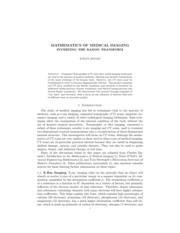
14KAILEY BOLLESModifying the indices of summation, this becomes (5)SMjpN 1NN 1XUk e2πijk/N k N MM1 XUk e2πijk/NNk 0The summations in equation (5) use the 2M 1 numbers UN M , .UN 1 , U0 , .UM .This method can be used to more generally approximate a Fourier series fˆ(ω)over a finite interval [0, 2πL]. Suppose that fˆ(ω) can be approximated within anacceptable tolerance, the definition of “acceptable” depending on application, byan integral over the interval [0, 2πL], that is, thatfˆ(ω) (6)Z f (x)e iωx dx Z2πf (x)e iωx dx.0If we subdivide [0, 2πL] into N subintervals of length 2πLN and choose partition,wherej 0,1,.,N,thenthelastintegralin equation (6) canpoints xj 2πjLNbe estimated byfˆ(ω) N 1 Xj 0If we let ω kL,2πjLN 2πjL 2πijLω/Nfe.Nwhere k is any integer, then we find that NX 1 k2πjL2πjL 2πijk/Nfˆ fe.LNNj 0This sampled Fourier transform is periodic of period N , but the actual values offˆ Lk are not, and so we again set the restriction that k N8 .For example, consider the function teh(t) 0for t 0,for t 0. To approximate ĥ Lk with a sampled Fourier transform, we (arbitrarily) chooseL 1, N 27 128. The sampled Fourier transform of h is therefore given bythe equation 127kπ X πj/64 πijk/64ĥ ee.L64 j 0Choosing a value of k such thatthatkL 3, we can calculate this approximation to find127ĥ (3)(7) π X πj/64 πijk/64ee64 j 0 0.12451 0.29884i.
MATHEMATICS OF MEDICAL IMAGING15The Fourier transform of h(t) isZĥ(ω) Z h(ξ)e iωξ dξe ξ e iωξ dξ01 iω1 ω2The Fourier transform for k 3 is therefore1 3iĥ(3) 0.1 0.3i.10Comparing this to the result of the sampled Fourier series in equation (7), we can seethat these results are remarkably similar. We could achieve an even more precisemodeling of ĥ Lk by choosing a larger value for N , but the calculations wouldrequire more time and computing power. Balancing between the precision of thesecalculations and the time taken to achieve them is vital to their uses in science andengineering, because too many calculations can quickly become prohibitive.If we calculate the sampled Fourier series for a several values of k, it is possiblefor us to make a graphical model of ĥ Lk . Figure 7 shows the Fourier transformand the sampled Fourier series of h(t) for k 0, ., 15. The sampled Fourier seriesare not in perfect agreement with the actual Fourier transform, but they do capturethe “general trend” of ĥ Lk . 8. The Radon Inversion FormulaThe inverse Radon transform is a technique used to reconstruct a function on theplane from its integrals over all lines in the plane. This provides a solution to theproblem of reconstructing an image of the body from CT scan data. Several methods for inverting the Radon transform exist, some of which use Fourier transforms,the Central Slice Theorem, and functional analysis. However, in “Elementary Inversion of Radon’s Transform” ([3]) Yves Nievergelt demonstrates proofs of thisformula using only calculus and basic linear algebra, though the other mathematicsexist as deeper, tacit portions of the formula and proof.In essence, this formula takes unfiltered backprojection a step further. Insteadof simply averaging the Radon transform over a line and “smearing” it to obtaina result, the inverse Radon transform R 1 (also called “filtered backprojection”)essentially applies an auxiliary filtering function, Γz , dependent upon t.Definition 8.1 (from [3]). Given any integrable function F of t and θ, the transform R* defines a function in x and yZ1 πR*F (x, y) : F (x cos θ y sin θ, θ) dθ.π 0The adjoint R*F (x, y) is equal to the average of F (t, θ) over the lines t,θ passingthrough the point (x, y).The relationship between the Radon transform R and its adjoint R* is verysimilar to that between the scalar product of vectors and a matrix and its transpose.
16KAILEY BOLLESFigure 7. The sampled Fourier series (black) and Fourier transform (red) of the function h. Image created using Maple.If we consider a continuous function f equal to zero outside some disc and anintegrable function F of t and θ, thenhRf, F i hf, R*F i.Proof. First consider the inner product of the Radon transform R and a functionF , both of which are in the space of (t, θ), such thatZ Z1 π hRf, F i Rf (t, θ)F (t, θ)dtdθ.π 0 Substituting in the definition of the Radon transform, find thatZ Z π Z 1F (t, θ)f (t cos θ s sin θ, t sin θ s cos θ)dsdtdθ.hRf, F i 0 π Switch the order of integration to giveZ Z Z π1hRf, F i f (t cos θ s sin θ, t sin θ s cos θ)F (t, θ)dθdsdt. π 0Changing coordinates from (t, θ) back to (x, y) via the substitutions x t cos θ s sin θ and y t sin θ s cos θ, the integral becomesZ Z Z1 πf (x, y)hRf, F i F (x cos θ y sin θ, θ)dθdxdy.π 0
MATHEMATICS OF MEDICAL IMAGING17Substitute in the definition of the adjoint R* to findZ Z f (x, y)R*F (x, y)dxdy hf, R*F i,hRf, F i thus exhibiting the equality between the inner product in the Radon transformline integral coordinate system (t, θ) and an inner product in the traditional planarcoordinate system (x, y). In order to introduce the inversion formula for the Radon transform, first considera simple notational convention. For every fixed vector K (κ, λ) in the plane, letfK be the translation of f by K. Therefore fK (x, y) f (x κ, y λ). This latterrelationship also leads to the fact thatR(fK )(ξ) Rf (ξ K).Proving this assertion requires the use of the Radon transform definition and ournew notation, asZ R(fK )(ξ) fK (t cos θ s sin θ, t sin θ s cos θ)dt Z f (κ t cos θ s sin θ, λ t sin θ s cos θ)dt Rf (ξ K). In order to derive the inversion formula, we will first approximate the functionf (x, y) by its average over a small disk D(X, z) of radius z centered at X (x, y).By the continuity of f assumed in the Radon transform,Z Z1f (x, y) limf (κ, λ)dκdλ.z 0 πz 2D(X,z)Let γz be the function equal to πz1 2 in the disk of radius z centered at the originD(0, z) and equal to zero outside this disk. ThenZ Z1fX (κ, λ)dκdλ lim hfX , γz i.f (x, y) fX (0, 0) limz 0z 0 πz 2D(X,z)Suppose the existence of some function Γz of t and θ such that γz R*Γz . Thenf (x, y) lim hfX , γz i lim hfX , R*Γz i lim hRfX , Γz i.z 0z 0z 0When expanded, the rightmost term provides us with a simple and useful formulafor the inverse Radon transform R 1 and proves that f is unique.Definition 8.2 (from [3]). The inverse Radon transform R 1 recovers a function f from the Radon transform Rf of that function. This inversion is given bythe formulaZ Z1 π f (x, y) limRf (t x cos θ y sin θ, θ)Γz (t)dtdθ.z 0 π 0 We must now find a function Γz that satisfies γz R*Γz . The function 2 for z t z, 1/(πz )Γz (t) 11for t z. πz2 1 2 21 z /tsatisfies this condition. In orde
The study of medical imaging has led to techniques vital to the practice of medicine, such as x-ray imaging, computed tomography (CT) scans, magnetic res-onance imaging, and a variety of other radiological imaging techniques. Such tech-niques allow the exam