Transcription
Downloaded from genome.cshlp.org on July 12, 2019 - Published by Cold Spring Harbor Laboratory PressMethodA novel approach for data integrationand disease subtypingTin Nguyen,1 Rebecca Tagett,2 Diana Diaz,2 and Sorin Draghici2,31Department of Computer Science and Engineering, University of Nevada, Reno, Nevada 89557, USA; 2Department of ComputerScience, Wayne State University, Detroit, Michigan 48202, USA; 3Department of Obstetrics and Gynecology, Wayne State University,Detroit, Michigan 48201, USAAdvances in high-throughput technologies allow for measurements of many types of omics data, yet the meaningful integration of several different data types remains a significant challenge. Another important and difficult problem is the discovery of molecular disease subtypes characterized by relevant clinical differences, such as survival. Here we present a novelapproach, called perturbation clustering for data integration and disease subtyping (PINS), which is able to address bothchallenges. The framework has been validated on thousands of cancer samples, using gene expression, DNA methylation,noncoding microRNA, and copy number variation data available from the Gene Expression Omnibus, the Broad Institute,The Cancer Genome Atlas (TCGA), and the European Genome-Phenome Archive. This simultaneous subtyping approachaccurately identifies known cancer subtypes and novel subgroups of patients with significantly different survival profiles.The results were obtained from genome-scale molecular data without any other type of prior knowledge. The approach issufficiently general to replace existing unsupervised clustering approaches outside the scope of bio-medical research, withthe additional ability to integrate multiple types of data.[Supplemental material is available for this article.]Once heralded as the holy grail, the capability of obtaining a comprehensive list of genes, proteins, or metabolites that are differentbetween disease and normal phenotypes is routine today. And yet,the holy grail of high-throughput has not delivered so far. Eventhough such high-throughput comparisons have become relatively easy to perform at a single level, integrating data of varioustypes in a meaningful way has become the new challenge of ourtime (Verhaak et al. 2010; The Cancer Genome Atlas ResearchNetwork 2011, 2012a,b,c, 2013, 2014, 2015; Yang et al. 2013;Davis et al. 2014; Hoadley et al. 2014; Robinson et al. 2015).Concurrently, we understand that many diseases, such ascancer, evolve through the interplay between the disease itselfand the host immune system (Coussens and Werb 2002; Yuet al. 2007). The treatment options, as well as the ultimate treatment success, are highly dependent on the specific tumor subtypefor any given stage (Choi et al. 2014; Lehmann and Pietenpol2014; Linnekamp et al. 2015). The challenge is to discover the molecular subtypes of disease and subgroups of patients.Cluster analysis has been a basic tool for subtype discovery using gene expression data. Agglomerative hierarchical clustering(HC) is a frequently used approach for clustering genes or samplesthat show similar expression patterns (Eisen et al. 1998; Alizadehet al. 2000; Perou et al. 2000). Other approaches, such as neuralnetwork–based methods (Kohonen 1990; Golub et al. 1999;Tamayo et al. 1999; Herrero et al. 2001; Luo et al. 2004), modelbased approaches (Ghosh and Chinnaiyan 2002; McLachlanet al. 2002; Jiang et al. 2004), matrix factorization (Brunet et al.2004; Gao and Church 2005), large-margin methods (Li et al.2009; Xu et al. 2004; Zhang et al. 2009), and graph-theoretical approaches (Ben-Dor et al. 1999; Hartuv and Shamir 2000; Sharanand Shamir 2000), have also been used. Arguably the state-of-Corresponding author: sorin@wayne.eduArticle published online before print. Article, supplemental material, and publication date are at 6.the-art approach in this area is consensus clustering (CC) (Montiet al. 2003; Wilkerson and Hayes 2010). CC develops a general,model-independent resampling-based methodology of class discovery and cluster validation (Ben-Hur et al. 2001; Dudoit andFridlyand 2002; Tseng and Wong 2005). Unfortunately, many approaches mentioned above are not able to combine multiple datatypes, and many attempts for subtype discovery based solely ongene expression have been undertaken but yielded only modestsuccess so far (very few gene expression tests are FDA approved).The goal of an integrative analysis is to identify subgroups ofsamples that are similar not only at one level (e.g., mRNA) but froma holistic perspective that can take into consideration phenomenaat various other levels (DNA methylation, miRNA, etc.). One strategy is to analyze each data type independently before combiningthem with the help of experts in the field (Verhaak et al. 2010;The Cancer Genome Atlas Research Network 2012a,b,c). However,this might lead to discordant results that are hard to interpret. Another approach, integrative phenotyping framework (iPF) (Kimet al. 2015), integrates multiple data types by concatenating allmeasurements to a single matrix and then clusters the patients using correlation distance and partitioning around medoids (PAM)(Kaufman and Rousseeuw 1987). This concatenation-based integration, however, further aggravates the “curse of dimensionality”(Bellman 1957). In turn, this leads to the use of gene filtering,which can introduce bias. Another challenge of this approach isidentifying the best way to concatenate multiple data types thatcome from different platforms (microarray, sequencing, etc.) anddifferent scales (Ritchie et al. 2015).Machine learning approaches, such as Bayesian CC (Lock andDunson 2013), MDI (Kirk et al. 2012), iCluster (Mo et al. 2013), 2017 Nguyen et al. This article is distributed exclusively by Cold SpringHarbor Laboratory Press for the first six months after the full-issue publicationdate (see http://genome.cshlp.org/site/misc/terms.xhtml). After six months, itis available under a Creative Commons License (Attribution-NonCommercial4.0 International), as described at 025–2039 Published by Cold Spring Harbor Laboratory Press; ISSN 1088-9051/17; www.genome.orgGenome Researchwww.genome.org2025
Downloaded from genome.cshlp.org on July 12, 2019 - Published by Cold Spring Harbor Laboratory PressNguyen et al.and iCluster (Shen et al. 2012, 2009), address the challenge of integration by using joint statistical modeling. They model the distribution of each data type and then maximize the likelihood of theobserved data. The recent iCluster makes an extra effort to reducethe parameter space by imposing sparse models, such as lasso(Tibshirani 1996). Though powerful, these approaches are limitedby their strong assumptions about the data and by the gene selection step used to reduce the computational complexity. Similaritynetwork fusion (SNF) (Wang et al. 2014) was the first approach thatallows for discovery of disease subtypes through integration of several types of high-throughput data on a genomic scale. SNF createsa fused network of patients using a metric fusion technique (Wanget al. 2012) and then partitions the data using spectral clustering(Von Luxburg 2007). SNF appears to be the state of the art in thisarea and has proven to be very powerful (Wang et al. 2014).However, the unstable nature of kernel-based clustering makesthe algorithm sensitive to small changes in molecular measurements or in its parameter settings.Here we propose a radically different integrative approach,perturbation clustering for data integration and disease subtyping(PINS), that addresses both challenges above: subtype discovery, aswell as integration of multiple data types. The algorithm is builtupon the resilience of patient connectivity and cluster ensembles(Strehl and Ghosh 2003) to ensure robustness against noise andbias. In an extensive analysis, we compare PINS with three subtyping algorithms that are selected to represent each of the main existing subtyping strategies: CC (Monti et al. 2003), SNF (Wanget al. 2014), and iCluster (Mo et al. 2013). CC is a resamplingbased approach that has been widely used for subtype discovery(Verhaak et al. 2010; The Cancer Genome Atlas ResearchNetwork 2011, 2012a,b,c, 2013, 2014, 2015; Yang et al. 2013;Davis et al. 2014; Hoadley et al. 2014). SNF is a graph-theoreticalapproach purported to allow discovery of disease subtypes basedon either a single data type or through integration of several datatypes. The third method, iCluster , is a model-based approachand is the enhanced version iCluster (Shen et al. 2009, 2012)and iCluster2 (Shen et al. 2013).ResultsHere, we first present the workflow to construct the optimal connectivity and the results obtained on a single data type. We thendescribe the two-stage procedure to address the challenge of integrating multiple types of data and the results obtained on cancerdiseases by integrating mRNA, miRNA, methylation, and copynumber variation (CNV) data. We compare the proposed approachwith these state-of-the-art methods on eight gene expression datasets involving a total of 12 tissues types and over 1000 samples. Ineach of these data sets, we show that PINS is better able to retrieveknown subtypes. In order to compare the data integration abilitiesof these four approaches, we also applied them to eight cancer datasets, involving mRNA, methylation, miRNA, and CNV data. Theseresults also show that PINS is better able to discover subtypesthat have significant survival differences compared with existingapproaches.Discovering subtypes based on a single data typeThe approach is based on the observation that differences arenaturally present between individuals, even in the most homogeneous population. Therefore, we hypothesize that if true subtypes2026Genome Researchwww.genome.orgof a disease do exist, they should be stable with respect to smallchanges in the features that we measure.We will describe this approach using an illustrative exampleshown in Figure 1A. In this simulated data set, we have three distinct classes of patients in which each class has a different set of differentially expressed genes (DEGs). Without any loss of generality,the genes are ordered such that the DEGs in the first class are plotted first (1–100), the DEGs in the second class are plotted second(101–200), etc. In order to find subtypes, we repeatedly perturbthe data (by adding Gaussian noise) and partition the samples/patients using any classical clustering algorithm (by default k-means,repeated 200 times). We test a range of potential cluster numbers k(by default k [2.10]) and identify the partitioning that is least affected by such perturbations. We then assess the cluster stability bycomparing the partitionings obtained from the original data tothose found with perturbed data for any given k. To quantify thesedifferences, we first construct a binary connectivity matrix, inwhich the element (i, j) represents the connectivity between patients i and j, and is equal to 1 (blue) if they belong to the same cluster, and 0 (white) otherwise. The upper parts in Figure 1, B throughE, show the original connectivity. The middle parts of the samepanels show the average connectivity for k [2.5] over the 200 trials. Next, we calculate the absolute difference between the originaland the perturbed connectivity matrices and compute the empirical cumulative distribution functions (CDFs) of the entries ofthe difference matrix (CDF-DM) (Fig. 1F). The area under thisCDF-DM curve (AUC) is used to assess the stability of the clustering. Figure 1G shows the behavior of the AUC (red curve), as thenumber of clusters varies from two to 10. In the ideal case of perfectly stable clusters, the original and perturbed connectivity matrices are identical, yielding a difference matrix of zeros, a CDFDM that jumps from zero to one at the origin, and an AUC ofone. Based on this criterion, we chose the partitioning with thehighest AUC. As shown in Figure 1G, the correct number of subtypes is three, as this corresponds to the largest AUC. The connectivity corresponding to this partitioning is considered the optimalconnectivity, which will serve as input for data integration.Interestingly, the perturbed connectivity matrices (middleparts of Fig. 1B–E) clearly suggest that there are three distinct classes of patients. This demonstrates that for truly distinct subtypesthe true connectivity between patients within each class is recovered when the data are perturbed, no matter how we set the valueof k. This resilience of patient connectivity occurs consistently regardless of the clustering algorithm being used (e.g., k-means, HC,or PAM) or the distribution of the data. When there are no trulydistinct subtypes, the connectivity is randomly distributed(Supplemental Fig. S2). When the number of true classes changes,the perturbed connectivity always reflects the true structure of thedata (Supplemental Figs. S2–S7).One of the disadvantages of existing clustering approaches,such as k-means, is that they will produce k clusters even forcompletely random data. The question is whether this artificiallyforced partitioning will also translate to the proposed approach.In order to demonstrate that this is not the case, we show theCDF-DM curves for completely random data as the black curvesin the lower panels of Figure 1, B through E. For each case of k {2, 4, 5}, the red curve (Dataset3) and the black curve (randomdata) are close to each other, reflecting that the perturbed connectivity for Dataset3 is almost as unstable as that of data without anystructure. In contrast, for the correct number of clusters (k 3) thered curve is far from the black curve, indicating that the clusteringobtained for this number of clusters is very different from random.
Downloaded from genome.cshlp.org on July 12, 2019 - Published by Cold Spring Harbor Laboratory PressData integration and disease subtypingFigure 1. The PINS algorithm applied on a single data type, using the simulated data named Dataset3. (A) The data set consists of 100 patients and threesubtypes, each having a different set of 100 differentially expressed genes. The numbers of patients in each subtype are 33, 33, and 34, respectively. (B–E)Original connectivity matrix (top), perturbed connectivity matrix (middle), and CDF of the difference matrix (bottom) for k 2, 3, 4, and 5, respectively. (F )CDF of the difference matrix (CDF-DM) for k [2.10]. (G) AUC values for Dataset3 (red curve), random data (black curve), and the difference (blue) between the two curves.Figure 1G contrasts the behavior of the AUC for Dataset3 againstthat of random data for all values of k from two to 10. The redand black curves show the AUC values for Dataset3 and randomdata, whereas the blue curve displays the difference (ΔAUC) between the two sets of AUC for k [2.10].In summary, the number of subtypes present in the data canbe identified based on any of the following three equivalent criteria: (1) the best (closest to upper left corner) CDF-DM (see Fig. 1F),(2) the highest AUC value (the peak of the red curve in Fig. 1G), or(3) the maximum difference between the AUC constructed fromthe data and the AUCs of random data (the peak of the blue curvein Fig. 1G).Results on gene expression data (single data type)In order to validate this approach, we tested it first using real datawith known subtypes. Also, we first start by using a single datatype. In order to do this, we used eight gene expression data sets,selected to include many samples (more than 1000), a large varietyof conditions and tissues, and a varied number of known subtypes.Genome Researchwww.genome.org2027
Downloaded from genome.cshlp.org on July 12, 2019 - Published by Cold Spring Harbor Laboratory PressNguyen et al.To address the particular challenge posed by situations in which asubtype is poorly represented in the data, we include both balanced data sets with a ratio of almost 1:1 between the numberof samples in the smallest and the largest subtype, as well as unbalanced sets with ratios between 1:3 and 1:33. We also note thatsome of these data sets were used in the publication of classicalsubtyping procedures, such as CC (Monti et al. 2003) and nonnegative matrix factorization (Brunet et al. 2004).Five of the data sets, GSE10245 (Kuner et al. 2009), GSE19188(Hou et al. 2010), GSE43580 (Tarca et al. 2013), GSE14924 (LeDieu et al. 2009), and GSE15061 (Mills et al. 2009), were downloaded from Gene Expression Omnibus, while the other threedata sets were downloaded from the Broad Institute: AML2004(Golub et al. 1999; Brunet et al. 2004), Lung2001 (Bhattacharjeeet al. 2001), and Brain2002 (Pomeroy et al. 2002). See theMethods section and Supplemental Table S1 for more details ofthese eight data sets.Since the true disease subtypes are known in these data sets, weuse the Rand Index (RI) (Rand 1971) and Adjusted Rand Index (ARI)(Hubert and Arabie 1985) to assess the performance of the resultedsubtypes. RI measures the agreement between a given clustering Nand the ground truth. In short, RI (a b)/, where a is the2number of pairs that belong to the same true subtype and are clustered together, b is the number of pairs that belong to different true Nsubtypes and are not clustered together, andis the number of2possible pairs that can be formed from the N samples. Intuitively,RI is the fraction of pairs that are grouped in the same way (eithertogether or not) in the two partitions compared (e.g., 0.9 means90% of pairs are grouped in the same way). The ARI is the corrected-for-chance version of the RI. The ARI takes values from 1 to1, with the ARI expected to be zero for a random subtyping.Table 1 shows the clustering results of PINS, CC, SNF, andiCluster for the eight gene expression data sets. Cells highlightedin green have the highest RI and ARI in their respective rows. For alleight data sets, PINS considerably outperforms existing approachesin identifying the known subtypes of each disease. More specifically, PINS yields the highest RI and ARI values for every singledata set tested.To assess the stability of the clustering algorithms, we also analyzed the gene expression data sets using different parameters forPINS, SNF, and iCluster . We demonstrate that PINS is robust tothe perturbation magnitude, while SNF and iCluster are very sensitive to their parameters (Supplemental Tables S3–S5). In addi-tion, PINS is also the most reliable when the signal to noise ratiodiminishes (Supplemental Fig. S8; Supplemental Table S2). Timecomplexity for each of the subtyping methods is reported inSupplemental Table S14 and Supplemental Figure S17.Integrating multiple types of dataThe challenge of integrating multiple types of data is addressed intwo stages. In the first stage, we identify subgroups of patients thatare strongly connected across heterogeneous data types. In the second stage, we analyze each subgroup to decide whether or not itmay warrant further splitting.Let us consider T data types from N patients. In the first stage,PINS works with each data type to build T connectivity matrices,one for each data type. A connectivity matrix can be representedas a graph, with patients as nodes and with connectivity betweenpatients as edges. Our goal is to identify subgraphs that are stronglyconnected across all data types. We merge the T connectivity matrices into a combined similarity matrix that represents the overallconnectivity between patients. This matrix is used as input for similarity-based clustering algorithms, such as HC, PAM (Kaufmanand Rousseeuw 1987), and Dynamic Tree Cut (Langfelder et al.2008). By default, we use all three algorithms to partition the patients and then choose the partitioning that agrees the mostwith the partitionings of individual data types (Strehl and Ghosh2003). This completes stage I. Since a very strong signal may dominate the clustering in stage I, we next consider each group one at atime and decide whether to split it further. A group may be splitagain if the data types are separable according to gap statistics(Tibshirani et al. 2001), and the stage I clustering is extremely unbalanced with low normalized entropy (for details, see Methods)(Cover and Thomas 2012)We illustrate the two stages of the procedure on the kidney renal clear cell carcinoma (KIRC) data set from TCGA (Fig. 2). The input consists of sample-matched mRNA, methylation, and miRNAmeasurements (Fig. 2A–C). We first build the optimal connectivitybetween patients for each data type (Fig. 2D–F). We then constructthe similarity between patients that is consistent across all datatypes (Fig. 2G). Partitioning this similarity matrix results in threegroups of patients. Group 1 corresponds to the second largestblue square, while group 2 corresponds to the largest blue square.Group 3 includes all other patients.In stage II, we check each discovered group independently todecide if it can be further divided. As a result, only group 1 is furthersplit into two subgroups (Fig. 2H). The first PCA plot shows theTable 1. The performance of PINS, consensus clustering (CC), similarity network fusion (SNF), and iCluster in discovering subtypes from geneexpression dataData 4Lung2001AML2004Brain2002CCSNFiCluster r each data set (row), cells highlighted in green have the highest Rand Index (RI) and Adjusted Rand Index (ARI). For all eight data sets, PINS outperforms its competitors by having the highest RI and ARI. SNF produced an error for GSE14924, shown as an NA value.2028Genome Researchwww.genome.org
Downloaded from genome.cshlp.org on July 12, 2019 - Published by Cold Spring Harbor Laboratory PressData integration and disease subtypingFigure 2. Data integration and disease subtyping illustrated on the kidney renal clear cell carcinoma (KIRC) data set. (A–C) The input consists of threematrices that have the same set of patients but different sets of measurements. (D–F) The optimal connectivity between the samples for each data type. (G)The similarity between patients that are consistent across all data types. Partitioning this matrix results in three groups of patients. (H) Group 1 is further splitinto two subgroups in stage II. (I ) Kaplan-Meier survival curves of four subtypes after stage II splitting of group 1. The survival analysis indicates that the fourgroups discovered after stage II have significantly different survival profiles (Cox P-value 0.00013).connectivity between patients in group 1 using mRNA data, whilethe second and third PCA plots show that for methylation andmiRNA data, respectively. The connectivity reflects that this group1 consists of two subgroups of patients: subgroup “1-1” in whichpatients are strongly connected to each other’s across all the threedata types, and subgroup “1-2” in which patients are loosely connected to each other’s. Figure 2I displays the four groups discoveredby PINS. These groups have very different survival profiles.Subtyping by integrating mRNA, miRNA, and methylation dataWe analyzed six different cancers which have curated level-threedata, available at the TCGA website (https://cancergenome.nih.gov): KIRC, glioblastoma multiforme (GBM), acute myeloid leukemia (LAML), lung squamous cell carcinoma (LUSC), breast invasive carcinoma (BRCA), and colon adenocarcinoma (COAD). Weused mRNA expression, DNA methylation, and miRNA expressiondata for each of the six cancers. TCGA contains multiple platformfor each data type. We chose the platforms giving the largest set ofcommon tumor samples across the three data types while still using asingle platform for each data type. Table 2 shows more details ofthe six TCGA cancer data sets.For each cancer, we first analyze each data type independently and report the resulting subtypes. We then analyze the threedata types together. PINS and SNF take the three matrices as inputwithout any further processing. Since CC and maxSilhouette(Rousseeuw 1987) are not designed to integrate multiple datatypes, we concatenate the three data types for the integrativeanalysis. For iCluster , we used the 2000 features with largest median absolute deviation for each data type. For some cancers,iCluster is unable to analyze the microRNA data.We note that our approach focuses on maximizing the stability of the subtypes, based on cluster ensemble and connectivitysimilarity, instead of maximizing the Euclidean distance betweendiscovered subtypes. In order to compare the proposed approachwith the classical approach, we also include a clustering methodthat maximizes the silhouette index (Rousseeuw 1987). Forthis maxSilhouette method, we use k-means as the clustering algorithm and the silhouette index as the objective function to identifythe optimal number of clusters.Genome Researchwww.genome.org2029
Downloaded from genome.cshlp.org on July 12, 2019 - Published by Cold Spring Harbor Laboratory PressNguyen et al.Table 2. Description of the six data sets from The Cancer Genome Atlas (TCGA): kidney renal clear cell carcinoma (KIRC), glioblastoma multiforme (GBM), lung squamous cell carcinoma (LUSC), breast invasive carcinoma (BRCA), acute myeloid leukemia (LAML), and colon adenocarcinoma (COAD)Data seti) Sample no.Data typeii) Components 06224,454710Illumina HiSeq RNASeqHumanMethylation27Illumina GASeq miRNASeqHT HG-U133AHumanMethylation27Illumina HiSeq miRNASeqIllumina GASeq RNASeqHumanMethylation27Illumina GASeq miRNASeqHT HG-U133AHumanMethylation27Illumina GASeq miRNASeqIllumina HiSeq RNASeqV2HumanMethylation27Illumina GASeq miRNASeqIllumina GASeq RNASeqHumanMethylation27Illumina GASeq miRNASeqFor all data sets, we use TCGA-curated level three data of mRNA expression, DNA methylation, and mRNA expression.The subtypes identified by the four approaches are analyzedusing the Kaplan-Meier survival analysis (Supplemental Fig. S9–S14; Kaplan and Meier 1958), and their statistical significance is assessed using Cox regression (Table 3; Therneau and Grambsch2000). After data integration, CC finds groups with significant survival differences in two out of the six cancers: GBM (P 0.039) andLAML (P 0.035). SNF, iCluster , and maxSilhouette find subgroups with significantly different survival only for LAML (P 0.037, P 0.017, and P 0.032, respectively). In contrast, PINSidentifies groups that have statistically significant survival differences in five out of the six cancers—KIRC (P 10 4), GBM (P 8.7 10 5), LAML (P 0.0024), LUSC (P 0.0097), and BRCA (P 0.034), showing a clear advantage of PINS over this state-ofthe-art method.We also analyzed the subtypes discovered by the five methods using the concordance index (CI) and silhouette index (Supplemental Tables S6, S7). In terms of silhouette, maxSilhouetteoutperforms all existing methods in all but one case (23/24).This is expected because maxSilhouette aims to maximize the silhouette values. However, higher silhouette values do not necessarily translate into better clinical correlation, especially for dataintegration. As shown in Table 3, PINS finds subtypes with significantly different survival for five out of the six cancers, while themaxSilhouette method does so for only one. Similarly, in termsof CI, PINS outperforms maxSilhouette in all of the six cancers(for more discussion about Silhouette index, see SupplementalFigs. S15, S16; Supplemental Section 3.6).We also analyzed different combinations of the three datatypes, e.g., mRNA plus methylation, mRNA plus miRNA, andmethylation plus miRNA. Overall, PINS outperforms the otherfour methods across the three different combinations (Supplemental Table S8). To investigate how stable PINS is with respect to theagreement cutoff, we reran our analysis using five different cutoffs:0.4, 0.45, 0.5, 0.6, and 0.7 (Supplemental Table S9). In four out ofthe six data sets (GBM, LAML, LUCS, COAD), there is no changewhatsoever, when this threshold varies from 0.4 to 0.7. In the remaining two data sets (KIRC and BRCA), the results remain thesame in seven out of 10 cases. For KIRC, when the cutoff changesfrom 0.5 to 0.6, (i.e., increases our requirement for agreement),2030Genome Researchwww.genome.orgPINS does not split the female group in stage II anymore. The second case is BRCA, when the cutoff changes from 0.45 to 0.4. Withthe low agreement cutoff, PINS clusters the patients using thestrong similarity matrix when this matrix is not supported bythe majority of patient pairs. Overall, the results are stable with respect to the choice of this parameter. Furthermore, for all choicesof this parameter, the results obtained continue to be better thanthose obtained with CC, SNF, and iCluster .Notably, the six data sets illustrated here include several interesting cases. In the KIRC data, no single data type appears to carrysufficient information for any of the four methods to be able toidentify groups with significant survival differences. However,when the three data types are integrated and analyzed together,PINS is able to extract four groups with very significant survival differences (P 10 4). Note that none of the other algorithms are ableto identify groups with significantly different survival profiles forthis disease.Another interesting situation is that in which a single
on either a single data type or through integration of several data types. The third method, iCluster , is a model-based approach and is the enhanced version iCluster (Shen et al. 2009, 2012) and iCluster2 (Shen et al. 2013). Results Here, we first present the workflow to construct the optim