Transcription
CS 224D: Deep Learning for NLP11Lecture Notes: Part I22Spring 2016Course Instructor: Richard SocherAuthors: Francois Chaubard, RohitMundra, Richard SocherKeyphrases: Natural Language Processing. Word Vectors. Singular Value Decomposition. Skip-gram. Continuous Bag of Words(CBOW). Negative Sampling.This set of notes begins by introducing the concept of NaturalLanguage Processing (NLP) and the problems NLP faces today. Wethen move forward to discuss the concept of representing words asnumeric vectors. Lastly, we discuss popular approaches to designingword vectors.1Introduction to Natural Language ProcessingWe begin with a general discussion of what is NLP. The goal of NLPis to be able to design algorithms to allow computers to "understand"natural language in order to perform some task. Example tasks comein varying level of difficulty:Natural Language Processing taskscome in varying levels of difficulty:Easy Spell Checking Keyword Search Finding SynonymsEasyMedium Spell Checking Parsing information from websites,documents, etc. Keyword SearchHard Machine Translation Finding SynonymsMedium Semantic Analysis Coreference Question Answering Parsing information from websites, documents, etc.Hard Machine Translation (e.g. Translate Chinese text to English) Semantic Analysis (What is the meaning of query statement?) Coreference (e.g. What does "he" or "it" refer to given a document?) Question Answering (e.g. Answering Jeopardy questions).The first and arguably most important common denominatoracross all NLP tasks is how we represent words as input to any andall of our models. Much of the earlier NLP work that we will notcover treats words as atomic symbols. To perform well on most NLPtasks we first need to have some notion of similarity and difference
cs 224d: deep learning for nlp2between words. With word vectors, we can quite easily encode thisability in the vectors themselves (using distance measures such asJaccard, Cosine, Euclidean, etc).2Word VectorsThere are an estimated 13 million tokens for the English languagebut are they all completely unrelated? Feline to cat, hotel to motel?I think not. Thus, we want to encode word tokens each into somevector that represents a point in some sort of "word" space. This isparamount for a number of reasons but the most intuitive reason isthat perhaps there actually exists some N-dimensional space (suchthat N 13 million) that is sufficient to encode all semantics ofour language. Each dimension would encode some meaning thatwe transfer using speech. For instance, semantic dimensions mightindicate tense (past vs. present vs. future), count (singular vs. plural),and gender (masculine vs. feminine).So let’s dive into our first word vector and arguably the mostsimple, the one-hot vector: Represent every word as an R V 1 vectorwith all 0s and one 1 at the index of that word in the sorted englishlanguage. In this notation, V is the size of our vocabulary. Wordvectors in this type of encoding would appear as the following: 0001 0 0 1 0 0 , w a 0 , w at 1 , · · · wzebra 0 w aardvark . . . . . . . . 1000We represent each word as a completely independent entity. Aswe previously discussed, this word representation does not give usdirectly any notion of similarity. For instance,(whotel )T wmotel (whotel )T wcat 0So maybe we can try to reduce the size of this space from R V tosomething smaller and thus find a subspace that encodes the relationships between words.3SVD Based MethodsFor this class of methods to find word embeddings (otherwise knownas word vectors), we first loop over a massive dataset and accumulate word co-occurrence counts in some form of a matrix X, and thenperform Singular Value Decomposition on X to get a USV T decomposition. We then use the rows of U as the word embeddings for allOne-hot vector: Represent every wordas an R V 1 vector with all 0s and one1 at the index of that word in the sortedenglish language.Fun fact: The term "one-hot" comesfrom digital circuit design, meaning "agroup of bits among which the legalcombinations of values are only thosewith a single high (1) bit and all theothers low (0)".
cs 224d: deep learning for nlp3words in our dictionary. Let us discuss a few choices of X.3.1 Word-Document MatrixAs our first attempt, we make the bold conjecture that words thatare related will often appear in the same documents. For instance,"banks", "bonds", "stocks", "money", etc. are probably likely to appear together. But "banks", "octopus", "banana", and "hockey" wouldprobably not consistently appear together. We use this fact to builda word-document matrix, X in the following manner: Loop overbillions of documents and for each time word i appears in document j, we add one to entry Xij . This is obviously a very large matrix(R V M ) and it scales with the number of documents (M). So perhaps we can try something better.3.2 Window based Co-occurrence MatrixThe same kind of logic applies here however, the matrix X storesco-occurrences of words thereby becoming an affinity matrix. In thismethod we count the number of times each word appears inside awindow of a particular size around the word of interest. We calculatethis count for all the words in corpus. We display an example below.Let our corpus contain just three sentences and the window size be 1:1. I enjoy flying. Generate V V co-occurrencematrix, X.2. I like NLP. Apply SVD on X to get X USV T . Select the first k columns of U to geta k-dimensional word vectors.3. I like deep learning.The resulting counts matrix will then be:II like enjoyX deeplearningNLPf lying.Using Word-Word 010deep01001000learning00010001 NLP01000001f lying00100001.00001110 We now perform SVD on X, observe the singular values (the diagonal entries in the resulting S matrix), and cut them off at some indexk based on the desired percentage variance captured: ik 1 σi V i 1 σi ik 1 σi V i 1 σiindicates the amount ofvariance captured by the first kdimensions.
cs 224d: deep learning for nlpWe then take the submatrix of U1: V ,1:k to be our word embeddingmatrix. This would thus give us a k-dimensional representation ofevery word in the vocabulary.Applying SVD to X: V V X V V V u1 u2 · · · V 0σ2.σ1 0 . V ··· · · · V .v1v2. Reducing dimensionality by selecting first k singular vectors: V V X̂ V u1 u2 V kk ··· k σ1 0 .0σ2. ··· ··· k .Both of these methods give us word vectors that are more thansufficient to encode semantic and syntactic (part of speech) information but are associated with many other problems: The dimensions of the matrix change very often (new words areadded very frequently and corpus changes in size). The matrix is extremely sparse since most words do not co-occur. The matrix is very high dimensional in general ( 106 106 ) Quadratic cost to train (i.e. to perform SVD) Requires the incorporation of some hacks on X to account for thedrastic imbalance in word frequencySome solutions to exist to resolve some of the issues discussed above: Ignore function words such as "the", "he", "has", etc. Apply a ramp window – i.e. weight the co-occurrence count basedon distance between the words in the document. Use Pearson correlation and set negative counts to 0 instead ofusing just raw count.As we see in the next section, iteration based methods solve manyof these issues in a far more elegant manner.v1v2. 4
cs 224d: deep learning for nlp45Iteration Based MethodsLet us step back and try a new approach. Instead of computing andstoring global information about some huge dataset (which might bebillions of sentences), we can try to create a model that will be ableto learn one iteration at a time and eventually be able to encode theprobability of a word given its context.We can set up this probabilistic model of known and unknownparameters and take one training example at a time in order to learnjust a little bit of information for the unknown parameters based onthe input, the output of the model, and the desired output of themodel.At every iteration we run our model, evaluate the errors, andfollow an update rule that has some notion of penalizing the modelparameters that caused the error. This idea is a very old one datingback to 1986. We call this method "backpropagating" the errors (seeLearning representations by back-propagating errors.David E. Rumelhart, Geoffrey E. Hinton, and Ronald J.Williams (1988).)Context of a word:The context of a word is the set of Csurrounding words. For instance, theC 2 context of the word "fox" in thesentence "The quick brown fox jumpedover the lazy dog" is {"quick", "brown","jumped", "over"}.4.1 Language Models (Unigrams, Bigrams, etc.)First, we need to create such a model that will assign a probability toa sequence of tokens. Let us start with an example:"The cat jumped over the puddle."A good language model will give this sentence a high probabilitybecause this is a completely valid sentence, syntactically and semantically. Similarly, the sentence "stock boil fish is toy" should have a verylow probability because it makes no sense. Mathematically, we cancall this probability on any given sequence of n words:P ( w1 , w2 , · · · , w n )We can take the unary language model approach and break apartthis probability by assuming the word occurrences are completelyindependent:nP ( w1 , w2 , · · · , w n ) P ( wi )i 1However, we know this is a bit ludicrous because we know thenext word is highly contingent upon the previous sequence of words.And the silly sentence example might actually score highly. So perhaps we let the probability of the sequence depend on the pairwiseprobability of a word in the sequence and the word next to it. We callthis the bigram model and represent it as:Unigram model:nP ( w1 , w2 , · · · , w n ) P ( wi )i 1
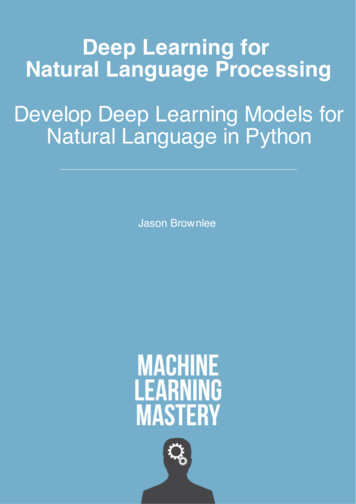
cs 224d: deep learning for nlp6nP ( w1 , w2 , · · · , w n ) P ( wi wi 1 )i 2Again this is certainly a bit naive since we are only concerningourselves with pairs of neighboring words rather than evaluating awhole sentence, but as we will see, this representation gets us prettyfar along. Note in the Word-Word Matrix with a context of size 1, webasically can learn these pairwise probabilities. But again, this wouldrequire computing and storing global information about a massivedataset.Now that we understand how we can think about a sequence oftokens having a probability, let us observe some example models thatcould learn these probabilities.Bigram model:nP ( w1 , w2 , · · · , w n ) P ( wi wi 1 )i 24.2 Continuous Bag of Words Model (CBOW)One approach is to treat {"The", "cat", ’over", "the’, "puddle"} as acontext and from these words, be able to predict or generate thecenter word "jumped". This type of model we call a Continuous Bagof Words (CBOW) Model.Let’s discuss the CBOW Model above in greater detail. First, weset up our known parameters. Let the known parameters in ourmodel be the sentence represented by one-hot word vectors. Theinput one hot vectors or context we will represent with an x (c) . Andthe output as y(c) and in the CBOW model, since we only have oneoutput, so we just call this y which is the one hot vector of the knowncenter word. Now let’s define our unknowns in our model.We create two matrices, V Rn V and U R V n . Where nis an arbitrary size which defines the size of our embedding space.V is the input word matrix such that the i-th column of V is the ndimensional embedded vector for word wi when it is an input to thismodel. We denote this n 1 vector as vi . Similarly, U is the outputword matrix. The j-th row of U is an n-dimensional embedded vectorfor word w j when it is an output of the model. We denote this row ofU as u j . Note that we do in fact learn two vectors for every word wi(i.e. input word vector vi and output word vector ui ).CBOW Model:Predicting a center word form thesurrounding contextNotation for CBOW Model: wi : Word i from vocabulary V V Rn V : Input word matrix vi : i-th column of V , the input vectorrepresentation of word wi U Rn V : Output word matrix ui : i-th row of U , the output vectorrepresentation of word wiWe breakdown the way this model works in these steps:1. We generate our one hot word vectors (x (c m) , . . . , x (c 1) , x (c 1) , . . . , x (c m) )for the input context of size m.2. We get our embedded word vectors for the context (vc m V x (c m) , vc m 1 V x (c m 1) , . . ., vc m V x (c m) )
cs 224d: deep learning for nlp3. Average these vectors to get v̂ 7vc m vc m 1 . vc m2m4. Generate a score vector z U v̂5. Turn the scores into probabilities ŷ softmax(z)6. We desire our probabilities generated, ŷ, to match the true probabilities, y, which also happens to be the one hot vector of theactual word.So now that we have an understanding of how our model wouldwork if we had a V and U , how would we learn these two matrices?Well, we need to create an objective function. Very often when weare trying to learn a probability from some true probability, we lookto information theory to give us a measure of the distance betweentwo distributions. Here, we use a popular choice of distance/lossmeasure, cross entropy H (ŷ, y).The intuition for the use of cross-entropy in the discrete case canbe derived from the formulation of the loss function: V H (ŷ, y) y j log(ŷ j )j 1Let us concern ourselves with the case at hand, which is that y isa one-hot vector. Thus we know that the above loss simplifies tosimply:H (ŷ, y) yi log(ŷi )In this formulation, c is the index where the correct word’s onehot vector is 1. We can now consider the case where our prediction was perfect and thus ŷc 1. We can then calculate H (ŷ, y) 1 log(1) 0. Thus, for a perfect prediction, we face no penalty orloss. Now let us consider the opposite case where our prediction wasvery bad and thus ŷc 0.01. As before, we can calculate our loss tobe H (ŷ, y) 1 log(0.01) 4.605. We can thus see that for probability distributions, cross entropy provides us with a good measure ofdistance. We thus formulate our optimization objective as:minimize J log P(wc wc m , . . . , wc 1 , wc 1 , . . . , wc m ) log P(uc v̂) logexp(ucT v̂) V j 1 exp(u Tj v̂) V ucT v̂ log exp(u Tj v̂)j 1We use gradient descent to update all relevant word vectors uc andvj.Figure 1: This image demonstrates howCBOW works and how we must learnthe transfer matrices
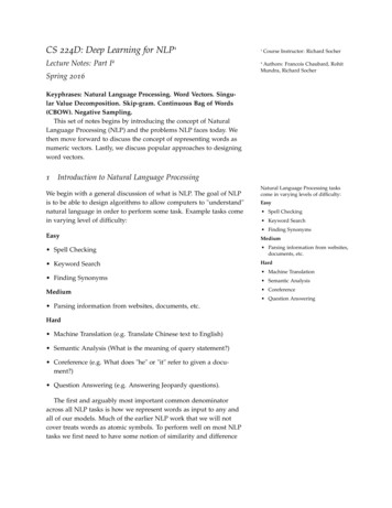
cs 224d: deep learning for nlp84.3 Skip-Gram ModelAnother approach is to create a model such that given the centerword "jumped", the model will be able to predict or generate thesurrounding words "The", "cat", "over", "the", "puddle". Here we callthe word "jumped" the context. We call this type of model a SkipGram model.Let’s discuss the Skip-Gram model above. The setup is largely thesame but we essentially swap our x and y i.e. x in the CBOW arenow y and vice-versa. The input one hot vector (center word) we willrepresent with an x (since there is only one). And the output vectorsas y( j) . We define V and U the same as in CBOW.Skip-Gram Model:Predicting surrounding context wordsgiven a center wordNotation for Skip-Gram Model: wi : Word i from vocabulary V V Rn V : Input word matrix vi : i-th column of V , the input vectorrepresentation of word wi U Rn V : Output word matrix ui : i-th row of U , the output vectorrepresentation of word wiWe breakdown the way this model works in these 6 steps:1. We generate our one hot input vector x2. We get our embedded word vectors for the context vc V x3. Since there is no averaging, just set v̂ vc ?4. Generate 2m score vectors, uc m , . . . , uc 1 , uc 1 , . . . , uc m usingu U vc5. Turn each of the scores into probabilities, y softmax(u)6. We desire our probability vector generated to match the true probabilities which is y(c m) , . . . , y(c 1) , y(c 1) , . . . , y(c m) , the one hotvectors of the actual output.As in CBOW, we need to generate an objective function for us toevaluate the model. A key difference here is that we invoke a NaiveBayes assumption to break out the probabilities. If you have notseen this before, then simply put, it is a strong (naive) conditionalindependence assumption. In other words, given the center word, alloutput words are completely independent.Figure 2: This image demonstrates howSkip-Gram works and how we mustlearn the transfer matrices
cs 224d: deep learning for nlpminimize J log P(wc m , . . . , wc 1 , wc 1 , . . . , wc m wc )2m logP ( wc m j wc )j 0,j6 m2m logP (uc m j vc )j 0,j6 m2mexp(ucT m j vc )j 0,j6 m k 1 exp(ukT vc ) log 2m j 0,j6 m V V ucT m j vc 2m log exp(ukT vc )k 1With this objective function, we can compute the gradients withrespect to the unknown parameters and at each iteration updatethem via Stochastic Gradient Descent.4.4 Negative SamplingLets take a second to look at the objective function. Note that thesummation over V is computationally huge! Any update we do orevaluation of the objective function would take O( V ) time whichif we recall is in the millions. A simple idea is we could instead justapproximate it.For every training step, instead of looping over the entire vocabulary, we can just sample several negative examples! We "sample" froma noise distribution (Pn (w)) whose probabilities match the orderingof the frequency of the vocabulary. To augment our formulation ofthe problem to incorporate Negative Sampling, all we need to do isupdate the: objective function gradients update rulesMikolov et al. present Negative Sampling in DistributedRepresentations of Words and Phrases and their Compositionality. While negative sampling is based on the Skip-Grammodel, it is in fact optimizing a different objective. Consider a pair(w, c) of word and context. Did this pair come from the trainingdata? Let’s denote by P( D 1 w, c) the probability that (w, c) camefrom the corpus data. Correspondingly, P( D 0 w, c) will be the9
cs 224d: deep learning for nlpprobability that (w, c) did not come from the corpus data. First, let’smodel P( D 1 w, c) with the sigmoid function:P( D 1 w, c, θ ) 1T1 e( vc vw )Now, we build a new objective function that tries to maximize theprobability of a word and context being in the corpus data if it indeed is, and maximize the probability of a word and context notbeing in the corpus data if it indeed is not. We take a simple maximum likelihood approach of these two probabilities. (Here we take θto be the parameters of the model, and in our case it is V and U .)θ argmaxθ argmaxθ argmaxθ argmaxθ argmaxθ P( D 1 w, c, θ ) P( D 1 w, c, θ ) log P( D 1 w, c, θ ) log11 log(1 )Tv )Tv )1 exp( uw1 exp( uwcc(w,c) D̃ log11 log()Tv )Tv )1 exp( uw1 exp(uwcc(w,c) D̃(w,c) D P( D 0 w, c, θ ) (1 P( D 1 w, c, θ ))(w,c) D̃(w,c) D(w,c) D̃(w,c) D(w,c) D(w,c) D log(1 P( D 1 w, c, θ ))(w,c) D̃Note that D̃ is a "false" or "negative" corpus. Where we would havesentences like "stock boil fish is toy". Unnatural sentences that shouldget a low probability of ever occurring. We can generate D̃ on the flyby randomly sampling this negative from the word bank. Our newobjective function would then be:log σ (ucT m j · vc ) K log σ( ũkT · vc )k 1In the above formulation, {ũk k 1 . . . K } are sampled from Pn (w).Let’s discuss what Pn (w) should be. While there is much discussionof what makes the best approximation, what seems to work best isthe Unigram Model raised to the power of 3/4. Why 3/4? Here’s anexample that might help gain some intuition:is: 0.93/4 0.92Constitution: 0.093/4 0.16bombastic: 0.013/4 0.032"Bombastic" is now 3x more likely to be sampled while "is" onlywent up marginally.10
Keyphrases: Natural Language Processing. Word Vectors. Singu-lar Value Decomposition. Skip-gram. Continuous Bag of Words (CBOW). Negative Sampling. This set of notes begins by introducing the concept of Natural Language Processing (NLP) and the problems NLP faces today. We then move fo