WIXLIB

WHITE PAPER UNDERSTANDING TIME CURRENT CURVESUnderstandingTime Current CurvesDavid Paul P.E., Engineering Design Manager,MAVERICK TechnologiesA time current curve (TCC) plots theinterrupting time of an overcurrentdevice based on a given current level.These curves are provided by themanufacturers of electrical overcurrentinterrupting devices such as fuses andcircuit breakers. These curves are partof the product acceptance testingrequired by Underwriters Laboratories(UL) and other rating agencies.The shape of the curves is dictated by both the physicalconstruction of the device as well as the settings selectedin the case of adjustable circuit breakers. The timecurrent curves of a device are important for engineers tounderstand because they show graphically the responseof the device to various levels of overcurrent.The orange curve is the transformer damage curve.The green curves are the cable damage curves. Each oneof these items will be explained. The system representedby this curve is well coordinated and adequately protectedfrom damage. It also has minimal Arc Flash hazard categoryratings due to low instantaneous circuit breaker trip values.The One Line Diagram and TCC curve show a typical hypotheticalindustrial power system (Figure 2). There is a utility deliverypoint with power supplied at a medium voltage level (In thiscase 4160 volts), which feeds the primary side of a 2.5MVA powertransformer through a medium voltage fused switch containingan E class fuse. The 480 volt secondary side of the transformerfeeds a piece of low voltage power switchgear utilizing drawout low voltage power circuit breakers for the main and feedercircuit breakers. The TCC plot also displays the transformerand cable damage curves. These curves are based onaccepted industry consensus standards published byANSI (for the transformer) and ICEA (for the cables).The curves allow the power system engineer to graphicallyrepresent the selective coordination of overcurrent devicesin an electrical system. Modern power system designsoftware packages such as EasyPower, SKM Power Tools,and Etap contain graphical libraries of curves to allow thepower system engineer the ability to plot, analyze and printthe curves with minimal effort compared to the previousmethods used when coordinating a power system.TCC Item IdentificationThe TCC curves shown (Figure 1) plot the interrupting responsetime of a current interrupting device versus time. Current isshown on the horizontal axis using a logarithmic scale and isplotted as amps X 10X. Time is shown on the vertical axis usinga logarithmic scale and is plotted in seconds X 10X. The lightblue curve is a switchgear feeder circuit breaker curve.The violet curve is the switchgear main circuit breaker curve.The red curve is the transformer primary fuse curve.Figure 1: Typical Time Current Curve Plot1/6

WHITE PAPER UNDERSTANDING TIME CURRENT CURVESInterpreting the damage curves is fairly straightforward. Operatingconditions (overcurrent protection) must be kept to the left of thedamage curve to guarantee no permanent damage is done to thetransformer or cable in question (Figure 3). Operating conditionswhich allow operation to the right of the damage curve subject thedevice in question to currents that cause permanent irreversibledamage, a shortened lifespan and possible catastrophic failure.Therefore the overcurrent and circuit breaker coordination schemesmust take this into account during the initial design phase.Figure 2: The One Line Diagram shownin figure 2 is represented in the TCCCurve in figure 3There are two transformer damage curves (shown in orange), one isdashed and the other is solid. The solid damage curve is theunbalanced damage curve which takes into account a derating factorfor transformer winding type and fault type. The dashed damagecurve is the 100% rating curve with no derating consideration.The transformer inrush current is also plotted as a single point onthe TCC diagram. Again, as part of the initial design, the transformerinrush current must be to the left of the transformer primary fusecurve otherwise the fuse will open when the transformer is energized.These differences in the unbalanced and 100% damage curves canbe mitigated with additional protective relaying to allow the 100%curve to be used for power system design without the risk oftransformer damage.There are three cable damage curves (shown in green). There is one curvefor each cable represented on the one line diagram. As part of the initialdesign, the overcurrent interrupting device must limit the fault current tothe left of the damage curve to prevent permanent damage. The damagecurves for the cables are dependent on size, insulation typeand raceway configuration.The light blue curve represents the circuit breaker settings for the feedercircuit breaker. The lower portion of the curve (below .05 seconds or 3cycles on the time axis) is the instantaneous trip function. The purposeof the instantaneous trip is to trip the circuit breaker quickly with nointentional delay (no more than a few cycles) on high magnitude faultcurrents. This quick trip protects electrical distribution equipmentfrom damage and keeps arc flash hazard categories low. Clearly thesetype faults must be interrupted quickly and do not allow the systemto wait and see if the fault will self clear. The minimum instantaneoussetting determines the minimum trip setting for the circuit breaker.Figure 3: Selectively coordinatedelectrical power system. Major elementsof the time current curve are labeled.In the case shown above, the instantaneous setting is 2400 amps and themaximum value displayed is available fault current at the circuit breaker.Small changes in the instantaneous setting can result in significantchanges in the Arc Flash Hazard category, so this is a setting whichmust be carefully selected according to sound engineering principles.2/6

WHITE PAPER UNDERSTANDING TIME CURRENT CURVESThe next section of the curve moving up the time axis is determined by the short time settings. Short time settingscover the time range from 0.05 to 0.50 seconds (3 to 30 cycles). The purpose of short time settings is to allow a timebased delay to elapse before tripping the circuit breaker for moderate current faults. This allows moderate faults time toclear themselves without tripping the circuit breaker. Examples of these types of overcurrents would be the inrush on alarge motor starting or a transformer inrush when it is first energized. The short time pickup setting shifts the curve onthe current axis. Increasing the short time pickup settings shifts the curve to the right and conversely lower settings shiftthe curve to the left. The short time delay setting moves the “knee” of the curve vertically on the time axis. Increasingthe short time delay setting moves the “knee” vertically up the time axis. Similarly, decreasing the settings moved the“knee” lower on the vertical axis. The described curve shifts are depicted on the TCC plots below. (Figures 4 - 7)Figure 4: Short Time Base CaseSTPU 2.5 ST DLY MinFigure 5: Decreased Short Time PickupNotice curve shift to left STPU 1.5Figure 6: Increased Short Time PickupNotice curve shift to Right STPU 4Figure 7: Increased Short Time DelayNotice curve shift vertically ST DLY Max3/6

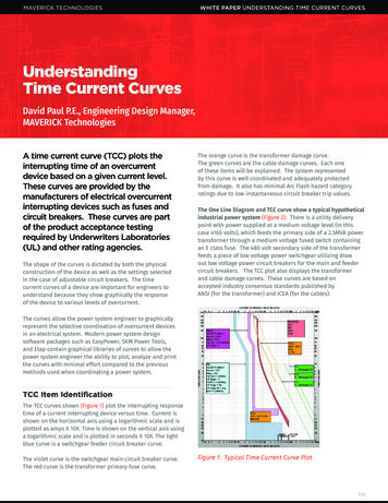
WHITE PAPER UNDERSTANDING TIME CURRENT CURVESThe next section of the curve moving up the time axis is the long time section. Long time settings cover the time range from0.5 to 1000 seconds. The purpose of long time settings is to allow a time-based delay to elapse before tripping the circuitbreaker for low level current faults. This allows low level faults time to clear themselves and allows electrical equipment tooperate in a temporarily overloaded condition provided it will not produce permanent damage to the equipment. Examplesof these types of overcurrents would be the overloading of a power transformer or large motor for a few minutes. The longtime pickup setting sets the ultimate trip value of the circuit breaker. Generally circuit breakers are set at their maximumlong time setting and cannot exceed the rating of the circuit breaker. They can be set at reduced values, which shiftsthe curve to the left on the current axis. There is also “knee” in the long time portion of the curve. The long time “knee”can be shifted up the time axis by increasing the long time delay setting. Conversely, the “knee” can be shifted lower bydecreasing the long term delay setting. The described curve shifts are depicted on the TCC plots below. (Figures 8 - 11)Figure 8: Long Time Base CaseTrip 800 AFigure 9: Long Time Delay IncreasedFigure 10: Long Time Delay DecreasedFigure 11: Long Time PickupDecreased Trip 400 A4/6

WHITE PAPER UNDERSTANDING TIME CURRENT CURVESAnother factor to notice in the curves is that they have a width to them. This is due to tolerance of the trip elementsin the circuit breaker. The curves below (Figures 12 and 13), will show the differences in this deadbandfor the same circuit breaker using an electronic versus non-electronic trip mechanism.Figure 12: Feeder Circuit Breaker withElectronic trip unit Microversa TripRMS-9 GE AKR series LVPCBFigure 13: Feeder Circuit Breakerwith Non-Electronic Trip EC-2 GEAKR series LVPCBNotice the difference in the tolerance in the trip curve of the feeder circuit breaker. The circuit breaker unit itself is thesame for both curves, so the tripping delays are constant. Settings for both trip units were set as similar as possible to eachother so performance could be easily compared. Notice there is more tolerance /- in the non-electronic trip unit due toanalog component tolerances and electro-mechanical devices inside the trip unit. The transition points on the electronictrip curve between instantaneous, short time and long time are much more distinct and accurate because of the digitalmicroprocessor-based trip. In the non-electronic trip, the transition points have time-based decay curves associated withthem due to the physics of the electro-mechanical trip elements. It is simply impossible to improve the performance of thenon-electronic trip because of the physical limits of the components. As can be seen in the above TCC curves, electronictrip units provide the engineer greater ability to accurately and selectively coordinate the electrical power system. Becauseof the obsolesce and lack of repair parts for older non-electronic trip units, the replacement of these units with electronictrip units can improve system coordination and reduce arc flash values in a properly designed electrical power system.Now that the basics of the TCC curves have been explained, a review of coordination is in order. Our sample curves to coordinatewill consist of an MCC with main 800 A fuses, a 1200 A feeder circuit breaker and the switchgear 3200 A main circuit breaker(Figures 14 - 15). In the uncoordinated system there is overlap of the circuit breaker trip curves, and in some instances themain circuit breaker will trip before the feeder circuit breaker. The main fuse in the MCC is also uncoordinated. While the fuseis not required, it is included in this example because it is typical of an industrial installation. The purpose of the fuse is toprovide current limiting to increase the short circuit withstand rating of the MCC bus. For example purposes, it is assumedthe MCC fuse is required and the cable feeder sizes cannot be changed. These assumptions make the example caserealistic as there are often constraints such as this found in real world coordination problems in industrial facilities.“Coordinated” means that selectivity between the feeder and the main circuit breaker is maintained. Per NationalElectric Code, “coordinated” is defined as “localization of an overcurrent condition to restrict outages to the circuit orequipment affected, accomplished by the choice of overcurrent protective devices and their ratings or settings.”5/6