Transcription
Renzo’s Math 490Introduction to TopologyTom BabinecChris BestMichael BlissNikolai BrendlerEric FuAdriane FungTyler KleinAlex LarsonTopcue LeeJohn MadonnaJoel MousseauNick PosavetzMatt RosenbergDanielle RogersAndrew SardoneJustin ShalerSmrithi SrinivasanPete TroyanJackson YimElizabeth UibleDerek Van FarowePaige WarmkerZheng WuNina ZhangWinter 2007
Mathematics 490 – Introduction to TopologyWinter 20072
Contents1 Topology91.1Metric Spaces . . . . . . . . . . . . . . . . . . . . . . . . . . . . . . . . . . . . . .91.2Open Sets (in a metric space) . . . . . . . . . . . . . . . . . . . . . . . . . . . . . 101.3Closed Sets (in a metric space) . . . . . . . . . . . . . . . . . . . . . . . . . . . . 111.4Topological Spaces . . . . . . . . . . . . . . . . . . . . . . . . . . . . . . . . . . . 111.5Closed Sets (Revisited) . . . . . . . . . . . . . . . . . . . . . . . . . . . . . . . . . 121.6Continuity . . . . . . . . . . . . . . . . . . . . . . . . . . . . . . . . . . . . . . . . 131.7Homeomorphisms . . . . . . . . . . . . . . . . . . . . . . . . . . . . . . . . . . . . 141.8Homeomorphism Examples . . . . . . . . . . . . . . . . . . . . . . . . . . . . . . 161.9Theorems On Homeomorphism . . . . . . . . . . . . . . . . . . . . . . . . . . . . 181.10 Homeomorphisms Between Letters of Alphabet . . . . . . . . . . . . . . . . . . . 191.10.1 Topological Invariants . . . . . . . . . . . . . . . . . . . . . . . . . . . . . 191.10.2 Vertices . . . . . . . . . . . . . . . . . . . . . . . . . . . . . . . . . . . . . 191.10.3 Holes . . . . . . . . . . . . . . . . . . . . . . . . . . . . . . . . . . . . . . 201.11 Classification of Letters . . . . . . . . . . . . . . . . . . . . . . . . . . . . . . . . 211.11.1 The curious case of the “Q” . . . . . . . . . . . . . . . . . . . . . . . . . . 221.12 Topological Invariants . . . . . . . . . . . . . . . . . . . . . . . . . . . . . . . . . 231.12.1 Hausdorff Property . . . . . . . . . . . . . . . . . . . . . . . . . . . . . . . 231.12.2 Compactness Property . . . . . . . . . . . . . . . . . . . . . . . . . . . . . 241.12.3 Connectedness and Path Connectedness Properties . . . . . . . . . . . . . 252 Making New Spaces From Old272.1Cartesian Products of Spaces . . . . . . . . . . . . . . . . . . . . . . . . . . . . . 272.2The Product Topology . . . . . . . . . . . . . . . . . . . . . . . . . . . . . . . . . 282.3Properties of Product Spaces . . . . . . . . . . . . . . . . . . . . . . . . . . . . . 293
Mathematics 490 – Introduction to TopologyWinter 20072.4Identification Spaces . . . . . . . . . . . . . . . . . . . . . . . . . . . . . . . . . . 302.5Group Actions and Quotient Spaces . . . . . . . . . . . . . . . . . . . . . . . . . 343 First Topological Invariants373.1Introduction . . . . . . . . . . . . . . . . . . . . . . . . . . . . . . . . . . . . . . . 373.2Compactness . . . . . . . . . . . . . . . . . . . . . . . . . . . . . . . . . . . . . . 373.2.1Preliminary Ideas . . . . . . . . . . . . . . . . . . . . . . . . . . . . . . . . 373.2.2The Notion of Compactness . . . . . . . . . . . . . . . . . . . . . . . . . . 403.3Some Theorems on Compactness . . . . . . . . . . . . . . . . . . . . . . . . . . . 433.4Hausdorff Spaces . . . . . . . . . . . . . . . . . . . . . . . . . . . . . . . . . . . . 473.5T1 Spaces . . . . . . . . . . . . . . . . . . . . . . . . . . . . . . . . . . . . . . . . 493.6Compactification . . . . . . . . . . . . . . . . . . . . . . . . . . . . . . . . . . . . 503.73.6.1Motivation . . . . . . . . . . . . . . . . . . . . . . . . . . . . . . . . . . . 503.6.2One-Point Compactification . . . . . . . . . . . . . . . . . . . . . . . . . . 503.6.3Theorems . . . . . . . . . . . . . . . . . . . . . . . . . . . . . . . . . . . . 513.6.4Examples . . . . . . . . . . . . . . . . . . . . . . . . . . . . . . . . . . . . 55Connectedness . . . . . . . . . . . . . . . . . . . . . . . . . . . . . . . . . . . . . 573.7.1Introduction . . . . . . . . . . . . . . . . . . . . . . . . . . . . . . . . . . 573.7.2Connectedness . . . . . . . . . . . . . . . . . . . . . . . . . . . . . . . . . 583.7.3Path-Connectedness . . . . . . . . . . . . . . . . . . . . . . . . . . . . . . 614 Surfaces634.1Surfaces . . . . . . . . . . . . . . . . . . . . . . . . . . . . . . . . . . . . . . . . . 634.2The Projective Plane . . . . . . . . . . . . . . . . . . . . . . . . . . . . . . . . . . 634.34.44.2.1RP2 as lines in R3 or a sphere with antipodal points identified. . . . . . . 634.2.2The Projective Plane as a Quotient Space of the Sphere . . . . . . . . . . 654.2.3The Projective Plane as an identification space of a disc . . . . . . . . . . 664.2.4Non-Orientability of the Projective Plane . . . . . . . . . . . . . . . . . . 69Polygons . . . . . . . . . . . . . . . . . . . . . . . . . . . . . . . . . . . . . . . . . 694.3.1Bigons . . . . . . . . . . . . . . . . . . . . . . . . . . . . . . . . . . . . . . 714.3.2Rectangles4.3.3Working with and simplifying polygons . . . . . . . . . . . . . . . . . . . 74. . . . . . . . . . . . . . . . . . . . . . . . . . . . . . . . . . . 72Orientability . . . . . . . . . . . . . . . . . . . . . . . . . . . . . . . . . . . . . . 764.4.1Definition . . . . . . . . . . . . . . . . . . . . . . . . . . . . . . . . . . . . 764
Mathematics 490 – Introduction to Topology4.54.64.7Winter 20074.4.2Applications To Common Surfaces . . . . . . . . . . . . . . . . . . . . . . 774.4.3Conclusion . . . . . . . . . . . . . . . . . . . . . . . . . . . . . . . . . . . 80Euler Characteristic . . . . . . . . . . . . . . . . . . . . . . . . . . . . . . . . . . 804.5.1Requirements . . . . . . . . . . . . . . . . . . . . . . . . . . . . . . . . . . 804.5.2Computation . . . . . . . . . . . . . . . . . . . . . . . . . . . . . . . . . . 814.5.3Usefulness . . . . . . . . . . . . . . . . . . . . . . . . . . . . . . . . . . . . 834.5.4Use in identification polygons . . . . . . . . . . . . . . . . . . . . . . . . . 83Connected Sums . . . . . . . . . . . . . . . . . . . . . . . . . . . . . . . . . . . . 854.6.1Definition . . . . . . . . . . . . . . . . . . . . . . . . . . . . . . . . . . . . 854.6.2Well-definedness . . . . . . . . . . . . . . . . . . . . . . . . . . . . . . . . 854.6.3Examples . . . . . . . . . . . . . . . . . . . . . . . . . . . . . . . . . . . . 874.6.4RP2 #T RP2 #RP2 #RP2 . . . . . . . . . . . . . . . . . . . . . . . . . . . 884.6.5Associativity . . . . . . . . . . . . . . . . . . . . . . . . . . . . . . . . . . 904.6.6Effect on Euler Characteristic . . . . . . . . . . . . . . . . . . . . . . . . . 90Classification Theorem . . . . . . . . . . . . . . . . . . . . . . . . . . . . . . . . . 924.7.1Equivalent definitions . . . . . . . . . . . . . . . . . . . . . . . . . . . . . 924.7.2Proof . . . . . . . . . . . . . . . . . . . . . . . . . . . . . . . . . . . . . . 935 Homotopy and the Fundamental Group975.1Homotopy of functions . . . . . . . . . . . . . . . . . . . . . . . . . . . . . . . . . 975.2The Fundamental Group . . . . . . . . . . . . . . . . . . . . . . . . . . . . . . . . 1005.35.45.2.1Free Groups . . . . . . . . . . . . . . . . . . . . . . . . . . . . . . . . . . 1005.2.2Graphic Representation of Free Group . . . . . . . . . . . . . . . . . . . . 1015.2.3Presentation Of A Group . . . . . . . . . . . . . . . . . . . . . . . . . . . 1035.2.4The Fundamental Group . . . . . . . . . . . . . . . . . . . . . . . . . . . . 103Homotopy Equivalence between Spaces . . . . . . . . . . . . . . . . . . . . . . . . 1055.3.1Homeomorphism vs. Homotopy Equivalence . . . . . . . . . . . . . . . . . 1055.3.2Equivalence Relation . . . . . . . . . . . . . . . . . . . . . . . . . . . . . . 1065.3.3On the usefulness of Homotopy Equivalence . . . . . . . . . . . . . . . . . 1065.3.4Simple-Connectedness and Contractible spaces . . . . . . . . . . . . . . . 107Retractions . . . . . . . . . . . . . . . . . . . . . . . . . . . . . . . . . . . . . . . 1085.4.1Examples of Retractions . . . . . . . . . . . . . . . . . . . . . . . . . . . . 1085
Mathematics 490 – Introduction to Topology5.5Computing the Fundamental Groups of Surfaces: The Seifert-Van Kampen Theorem . . . . . . . . . . . . . . . . . . . . . . . . . . . . . . . . . . . . . . . . . . . 1105.5.15.6Winter 2007Examples: . . . . . . . . . . . . . . . . . . . . . . . . . . . . . . . . . . . . 112Covering Spaces5.6.1. . . . . . . . . . . . . . . . . . . . . . . . . . . . . . . . . . . . 113Lifting . . . . . . . . . . . . . . . . . . . . . . . . . . . . . . . . . . . . . . 1176
Mathematics 490 – Introduction to TopologyWinter 2007What is this?This is a collection of topology notes compiled by Math 490 topology students at the Universityof Michigan in the Winter 2007 semester. Introductory topics of point-set and algebraic topologyare covered in a series of five chapters.Foreword (for the random person stumbling upon this document)What you are looking at, my random reader, is not a topology textbook. It is not the lecturenotes of my topology class either, but rather my student’s free interpretation of it. Well, Ishould use the word free with a little bit of caution, since they *had to* do this as their finalproject. These notes are organized and reflect tastes and choices of my students. I have doneonly a minimal amount of editing, to give a certain unity to the manuscript and to scrap outsome mistakes - and so I don’t claim merits for this work but to have lead my already greatstudents through this semester long adventure discovering a little bit of topology.Foreword (for my students)Well, guys, here it is! You’ve done it all, and here is a semester worth of labor, studying, buthopefully fun as well. I hope every once in a while you might enjoy flipping through the pagesof this book and reminiscing topology.and that in half a century or so you might be tellingexaggerated stories to your grandchildren about this class.A great thank to you all for a very good semester!7
Mathematics 490 – Introduction to TopologyWinter 20078
Chapter 1TopologyTo understand what a topological space is, there are a number of definitions and issues that weneed to address first. Namely, we will discuss metric spaces, open sets, and closed sets. Oncewe have an idea of these terms, we will have the vocabulary to define a topology. The definitionof topology will also give us a more generalized notion of the meaning of open and closed sets.1.1Metric SpacesDefinition 1.1.1. A metric space is a set X where we have a notion of distance. That is, ifx, y X, then d(x, y) is the “distance” between x and y. The particular distance function mustsatisfy the following conditions:1. d(x, y) 0 for all x, y X2. d(x, y) 0 if and only if x y3. d(x, y) d(y, x)4. d(x, z) d(x, y) d(y, z)To understand this concept, it is helpful to consider a few examples of what does and does notconstitute a distance function for a metric space.Example 1.1.2. For any space X, let d(x, y) 0 if x y and d(x, y) 1 otherwise.This metric, called the discrete metric, satisfies the conditions one through four.Example 1.1.3. The Pythagorean Theorem gives the most familiar notion of distance for pointsin Rn . In particular, when given x (x1 , x2 , ., xn ) and y (y1 , y2 , ., yn ), the distance f asvu nuXd(x, y) t (xi yi )2i 19
Mathematics 490 – Introduction to TopologyWinter 2007Example 1.1.4. Suppose f and g are functions in a space X {f : [0, 1] R}. Doesd(f, g) max f g define a metric?Again, in order to check that d(f, g) is a metric, we must check that this function satisfies theabove criteria. But in this case property number 2 does not hold, as can be shown by consideringtwo arbitrary functions at any point within the interval [0, 1]. If f (x) g(x) 0, this doesnot imply that f g because f and g could intersect at one, and only one, point. Therefore,d(f, g) is not a metric in the given space.1.2Open Sets (in a metric space)Now that we have a notion of distance, we can define what it means to be an open set in ametric space.Definition 1.2.1. Let X be a metric space. A ball B of radius r around a point x X isB {y X d(x, y) r}.We recognize that this ball encompasses all points whose distance is less than r from x .Definition 1.2.2. A subset O X is open if for every point x O, there is a ball around xentirely contained in O.Example 1.2.3. Let X [0, 1]. The interval (0, 1/2) is open in X.Example 1.2.4. Let X R. The interval [0, 1/2) is not open in X.With an open set, we should be able to pick any point within the set, take an infinitesimal stepin any direction within our given space, and find another point within the open set. In the firstexample, we can take any point 0 x 1/2 and find a point to the left or right of it, withinthe space [0, 1], that also is in the open set [0, 1). However, this cannot be done with the secondexample. For instance, if we take the point within the set [0, 1), say 0, and take an infinitesimalstep to the left while staying within our given space X, we are no longer within the set [0, 1).Therefore, this would not be an open set within R.If a set is not open, this does not imply that it is closed. Furthermore, there exists setsthat are neither open, nor closed, and sets that are open and closed.Lastly, open sets in spaces X have the following properties:1. The empty set is open2. The whole space X is open3. The union of any collection of open sets is open4. The intersection of any finite number of open sets is open.10
Mathematics 490 – Introduction to Topology1.3Winter 2007Closed Sets (in a metric space)While we can and will define a closed sets by using the definition of open sets, we first define itusing the notion of a limit point.Definition 1.3.1. A point z is a limit point for a set A if every open set U containing zintersects A in a point other than z.Notice, the point z could be in A or it might not be in A. The following example will help makethis clear.Example 1.3.2. Consider the open unit disk D {(x, y) : x2 y 2 1}. Any point in D is alimit point of D. Take (0, 0) in D. Any open set U about this point will contain other pointsin D. Now consider (1, 0), which is not in D. This is still a limit point because any open setabout (1, 0) will intersect the disk D.The following theorem and examples will give us a useful way to define closed sets, and will alsoprove to be very helpful when proving that sets are open as well.Definition 1.3.3. A set C is a closed set if and only if it contains all of its limit points.Example 1.3.4. The unit disk in the previous example is not closed because it does not containall of its limit points; namely, (1, 0).Example 1.3.5. Let A Z, a subset of R. This is a closed set because it does contain all ofits limit points; no point is a limit point! A set that has no limit points is closed, by default,because it contains all of its limit points.Every intersection of closed sets is closed, and every finite union of closed sets is closed.1.4Topological SpacesWe now consider a more general case of spaces without metrics, where we can still make senseof (or rather define appropriately) the notions of open and closed sets. These spaces are calledtopological spaces.Definition 1.4.1. A topological space is a pair (X, τ ) where X is a set and τ is a set ofsubsets of X satisfying certain axioms. τ is called a topology.Since this is not particularly enlightening, we must clarify what a topology is.Definition 1.4.2. A topology τ on a set X consists of subsets of X satisfying the followingproperties:1. The empty set and the space X are both sets in the topology.2. The union of any collection of sets in τ is contained in τ .3. The intersection of any finitely many sets in τ is also contained in τ .11
Mathematics 490 – Introduction to TopologyWinter 2007The following examples will help make this concept more clear.Example 1.4.3. Consider the following set consisting of 3 points; X {a, b, c} and determineif the set τ { , X, {a}, {b}} satisfies the requirements for a topology.This is, in fact, not a topology because the union of the two sets {a} and {b} is the set {a, b},which is not in the set τExample 1.4.4. Find all possible topologies on X {a, b}.1. , {a, b}2. , {a}, {a, b}3. , {b}, {a, b}4. , {a}, {b}, {a, b}The reader can check that all of these are topologies by making sure they follow the 3 propertiesabove. The first topology in the list is a common topology and is usually called the indiscretetopology; it contains the empty set and the whole space X. The following examples introducesome additional common topologies:Example 1.4.5. When X is a set and τ is a topology on X, we say that the sets in τ are open.Therefore, if X does have a metric (a notion of distance), then τ {all open sets as definedwith the ball above} is indeed a topology. We call this topology the Euclidean topology. It isalso referred to as the usual or ordinary topology.Example 1.4.6.If Y X and τx is a topology on X, one can define the Induced topologyTas τy {O Y O τx }.This last example gives one reason why we must only take finitely many intersections whendefining a topology.Example 1.4.7. Let X R with the usual topology. Then certainly in this standard Euclideantopology, ( 1/n, 1/n) is an open set for any integer n. However, the infinite intersectionT n 1 ( 1/n, 1/n) is the set containing just 0. Thus, it is a single point set, which is not openin this topology.1.5Closed Sets (Revisited)As promised, we can now generalize our definition for a closed set to one in terms of open setsalone which removes the need for limit points and metrics.Definition 1.5.1. A set C is closed if X C is open.Now that we have a new definition of a closed set, we can prove what used to be definition 1.3.3as a theorem: A set C is a closed set if and only if it contains all of its limit points.12
Mathematics 490 – Introduction to TopologyWinter 2007Proof. Suppose a set A is closed. If it has no limit points, there is nothing to check as it triviallycontains its limit points. Now suppose z is a limit point of A. Then if z A, it contains thislimit point. So suppose for the sake of contradiction that z is a limit point and z is not in A.Now we have assumed A was closed, so its complement is open. Since z is not in A, it is in thecomplement of A, which is open; which means there is an open set U containing z containedin the complement of A. This contradicts that z is a limit point because a limit point is, bydefinition, a point such that every open set about z meets A. Conversely, if A contains all itslimit points, then its complement is open. Suppose x is in the complement of A. Then it cannot be a limit point (by the assumption that A contains all of its limit points). So x is not alimit point which means we can find some open set around x that doesn’t meet A. This provesthe complement is open, i.e. every point in the complement has an open set around it thatavoids A.Example 1.5.2. Since we know the empty set is open, X must be closed.Example 1.5.3. Since we know that X is open, the empty set must be closed.Therefore, both the empty set and X and open and closed.1.6ContinuityIn topology a continuous function is often called a map. There are 2 different ideas we can useon the idea of continuous functions.Calculus StyleDefinition 1.6.1. f : Rn Rm is continuous if for every 0 there exists δ 0 such thatwhen x x0 δ then f (x) f (x0 ) .The map is continuos if for any small distance in the pre-image an equally small distance isapart in the image. That is to say the image does not “jump.”Topology StyleIn tpology it is necessary to generalize down the definition of continuity, because the notion ofdistance does not always exist or is different than our intuitive idea of distance.Definition 1.6.2. A function f : X Y is continuous if and only if the pre-image of any openset in Y is open in X.If for whatever reason you prefer closed sets to open sets, you can use the following equivalentdefinition:Definition 1.6.3. A function f : X Y is continuous if and only if the pre-image of anyclosed set in Y is closed in X.Let us give one more definition and then some simple consequences:13
Mathematics 490 – Introduction to TopologyWinter 2007Definition 1.6.4. Given a point x of X, we call a subset N of X a neighborhood of X if we canfind an open set O such that x O N .1. A function f : X Y is continuous if for any neighborhood V of Y there is a neighborhoodU of X such that f (U ) V .2. A composition of 2 continuous functions is continuous.Figure 1.1: Continuity of f with neighborhoods.1.7HomeomorphismsHomeomorphism is the notion of equality in topology and it is a somewhat relaxed notionof equality. For example, a classic example in topology suggests that a doughnut and coffeecup are indistinguishable to a topologist. This is because one of the geometric objects can bestretched and bent continuously from the other.The formal definition of homeomorphism is as follows.Definition 1.7.1. A homeomorphism is a function f : X Y between two topological spacesX and Y that is a continuous bijection, and has a continuous inverse function f 1 .14
Mathematics 490 – Introduction to TopologyWinter 2007Figure 1.2: Homeomorphism between a doughnut and a coffee cup.Another equivalent definition of homeomorphism is as follows.Definition 1.7.2. Two topological spaces X and Y are said to be homeomorphic if there arecontinuous map f : X Y and g : Y X such thatf g IYandg f IX .Moreover, the maps f and g are homeomorphisms and are inverses of each other, so we maywrite f 1 in place of g and g 1 in place of f .Here, IX and IY denote the identity maps.When inspecting the definition of homeomorphism, it is noted that the map is required to becontinuous. This means that points that are “close together” (or within an neighborhood, if ametric is used) in the first topological space are mapped to points that are also “close together”in the second topological space. Similar observation applies for points that are far apart.As a final note, the homeomorphism forms an equivalence relation on the class of all topological spaces. Reflexivity: X is homeomorphic to X. Symmetry: If X is homeomorphic to Y , then Y is homeomorphic to X. Transitivity: If X is homeomorphic to Y , and Y is homeomorphic to Z, then X is homeomorphic to Z.The resulting equivalence classes are called homeomorphism classes.15
Mathematics 490 – Introduction to Topology1.8Winter 2007Homeomorphism ExamplesSeveral examples of this important topological notion will now be given.Example 1.8.1. Any open interval of R is homeomorphic to any other open interval. ConsiderX ( 1, 1) and Y (0, 5). Let f : X Y be5f (x) (x 1).2Observe that f is bijective and continuous, being the compositions of addition and multiplication.Moreover, f 1 exists and is continuous:2f 1 (x) x 1.5Note that neither [0, 1] nor [0, 1) is homeomorphic to (0, 1) as such mapping between theseintervals, if constructed, will fail to be a bijection due to endpoints.Example 1.8.2. There exists homeomorphism between a bounded and an unbounded set. Suppose1f (x) .xThen it follows that (0, 1) and (1, ) are homeomorphic. It is interesting that we are able to“stretch” a set to infinite length.Example 1.8.3. Any open interval is, in fact, homeomorphic to the real line. Let X ( 1, 1)and Y R. From the previous example it is clear that the general open set (a, b) is homeomorphic to ( 1, 1). Now define a continuous map f : ( 1, 1) R by πx .f (x) tan2This continuous bijection possesses a continuous inverse f 1 : R ( 1, 1) byf 1 (x) 2arctan(x).πHence f : ( 1, 1) R is a homeomorphism.Example 1.8.4. A topologist cannot tell the difference between a circle S 1 {(x, y) R2 x2 y 2 1} and a square T {(x, y) R2 x y 1}, as there is a function f : S 1 Tdefined by yxf (x, y) , x y x y which is continuous, bijective, and has a continuous inversef 1 (x, y) xpx2 y 2y,px2 y 2!.Both circle and square are therefore topologically identical. S 1 and T are sometimes calledsimple closed curves (or Jordan curves).16
Mathematics 490 – Introduction to TopologyWinter 20072.5-5-4-3-2-1012345-2.5Figure 1.3: The graph of f 1 (x).Example 1.8.5. S 1 with a point removed is homeomorphic with R. Without loss of generality,suppose we removed the North Pole. Then the stereographic projection is a homeomorphismbetween the real line and the remaining space of S 1 after a point is omitted.Place the circle “on” the x-axis with the point omitted being directly opposite the real line. Moreprecisely, let S 1 {(x, y) R x2 (y 1/2)2 1/4} and suppose the North Pole is N (0, 1).Using geometry, we may construct f : S 1 \ N R by definingf (x, y) 2x.1 yf is well-defined and continuous as the domain of f excludes y 1, i.e. the North Pole. Withthe continuous inverse function 4x x2 4 1,,f (x) x2 4 x2 4we have f f 1 f 1 f I, hence f is a homeomorphism.Stereographic projection is a mapping that plays pivotal roles in cartography (mapmaking)and geometry. One interesting properties of stereographic projection is that this mapping isconformal, namely it preserves the angles at which curves cross each other.Example 1.8.6. The annulus A {(x, y) R2 1 x2 y 2 4} is homeomorphic to thecylinder C {(x, y, z) R3 x2 y 2 1, 0 z 1} since there exists continuous function17
Mathematics 490 – Introduction to TopologyWinter 2007Figure 1.4: Stereographic projection of S 2 \ N to R2 .f : C A and g : A Cf (x, y, z) ((1 z)x, (1 z)y)andg(x, y) xpx2 y 2y,p,x2 y 2!px2 y 2 1such that f g g f I. Thus f and g are homeomorphisms.1.9Theorems On HomeomorphismTheorem 1.9.1. If f : X Y is a homeomorphism and g : Y Z is another homeomorphism,then the composition g f : X Z is also a homeomorphism.Proof. We need to establish that g f is continuous and has a continuous inverse for it tobe a homeomorphism. The former is obvious as the composition of two continuous maps iscontinuous.Since f and g are homeomorphisms by hypothesis, there exists f 1 : Y X and g 1 : Z Ythat are continuous. By the same token, f 1 g 1 is continuous and (g f ) f 1 g 1 g f f 1 g 1 g g 1 IY . Similarly (f g) g 1 f 1 IX . Therefore g f is a homeomorphism.18
Mathematics 490 – Introduction to TopologyWinter 2007Various topological invariants will be discussed in Chapter 3, including connectedness, compactness, and Hausdorffness. Recall that homeomorphic spaces share all topological invariants.Hence the following theorem (without proof) immediately follows:Theorem 1.9.2. Let X and Y be homeomorphic topological spaces. If X is connected orcompact or Hausdorff, then so is Y .1.10Homeomorphisms Between Letters of AlphabetLetters of the alphabet are treated as one-dimensional objects. This means that the lines andcurves making up the letters have zero thickness. Thus, we cannot deform or break a singleline into multiple lines. Homeomorphisms between the letters in most cases can be extended tohomeomorphisms between R2 and R2 that carry one letter into another, although this is not arequirement – they can simply be a homeomorphism between points on the letters.1.10.1Topological InvariantsBefore classifying the letters of the alphabet, it is helpful to get a feel for the topologicalinvariants of one-dimensional objects in R2 . The number of 3-vertices, 4-vertices, (n-vertices,in fact, for n 3), and the number of holes in the object are the topological invariants whichwe have identified.1.10.2VerticesThe first topological invariant is the number and type of vertices in an object. We think of avertex as a point where multiple curves intersect or join together. The number of intersectingcurves determines the vertex type.Definition 1.10.1. An n-vertex in a subset L of a topological space S is an element v L suchthat there exists some neighborhood N0 S of v where all neighborhoods N N0 of v satisfythe following properties:1. N L is connected.2. The set formed by removing v from N L, i.e., {a N L a 6 v}, is not connected, andis composed of exactly n disjoint sets, each of which is connected.The definition of connectedness will be discussed much more in the course and will not be givenhere. Intuitively, though, a set is connected if it is all in one piece. So the definition of ann-vertex given above means that when we get close enough to an n-vertex, it looks like onepiece, and if we remove the vertex from that piece, then we get n separate pieces.We can say that for a given n 3, the number of n-vertices is a topological invariant becausehomeomorphisms preserve connectedness. Thus, the connected set around a vertex must mapto another connected set, and the set of n disjoint, connected pieces must map to another setof n disjoint connected pieces.19
Mathematics 490 – Introduction to TopologyWinter 2007The number of 2-vertices is not a useful topological invariant. This is true because every curvehas an infinite number of 2-vertices (every point on the curve not intersecting another curve isa 2-vertex). This does not help us to distinguish between classes of letters.Figure 1.5: 3-vertex homeomorphism exampleThree curves intersecting in a 3-vertex are homeomorphic to any other three curves intersectingin a 3-vertex. However, they are not homeomorphic to a single curve. This point is illustratedin Figure 1.5.Similarly, any set close to a 4-vertex is homeomorphic to any other set close to a 4-vertex. Inthis case, “close” means a small neighborhood in which there are no other n-vertices (n 3).Figure 1.6 shows an example of this.Figure 1.6: 4-vertex homeomorphism example1.10.3HolesIt is very clear when a one dimensional shape in two dimensional space has a hole: a shapepossessing a hole closes in on itself. As a result, a topological s
notes of my topology class either, but rather my student’s free interpretation of it. Well, I should use the word free with a little bit of caution, since they *had to* do this as their final project. These notes are organized