Transcription
Chapter 2The Solow Growth Model (and a lookahead)2.1Centralized Dictatorial Allocations In this section, we start the analysis of the Solow model by pretending that there isa dictator, or social planner, that chooses the static and intertemporal allocation ofresources and dictates that allocations to the households of the economy We will latershow that the allocations that prevail in a decentralized competitive market environment coincide with the allocations dictated by the social planner.2.1.1The Economy, the Households and the Dictator Time is discrete, t {0, 1, 2, .}. You can think of the period as a year, as a generation,or as any other arbitrary length of time. The economy is an isolated island. Many households live in this island. There are9
George-Marios Angeletosno markets and production is centralized. There is a benevolent dictator, or socialplanner, who governs all economic and social affairs. There is one good, which is produced with two factors of production, capital and labor,and which can be either consumed in the same period, or invested as capital for thenext period. Households are each endowed with one unit of labor, which they supply inelasticly tothe social planner. The social planner uses the entire labor force together with theaccumulated aggregate capital stock to produce the one good of the economy. In each period, the social planner saves a constant fraction s (0, 1) of contemporaneous output, to be added to the economy’s capital stock, and distributes the remainingfraction uniformly across the households of the economy. In what follows, we let Lt denote the number of households (and the size of the laborforce) in period t, Kt aggregate capital stock in the beginning of period t, Yt aggregateoutput in period t, Ct aggregate consumption in period t, and It aggregate investmentin period t. The corresponding lower-case variables represent per-capita measures: kt Kt /Lt , yt Yt /Lt , it It /Lt , and ct Ct /Lt .2.1.2Technology and Production The technology for producing the good is given byYt F (Kt , Lt )(2.1)where F : R2 R is a (stationary) production function. We assume that F iscontinuous and (although not always necessary) twice differentiable.10
Lecture Notes We say that the technology is “neoclassical ” if F satisfies the following properties1. Constant returns to scale (CRS), or linear homogeneity:F (µK, µL) µF (K, L), µ 0.2. Positive and diminishing marginal products:FK (K, L) 0,FKK (K, L) 0,FL (K, L) 0,FLL (K, L) 0.where Fx F/ x and Fxz 2 F/( x z) for x, z {K, L}.3. Inada conditions:lim FK lim FL ,K 0L 0lim FK K lim FL 0.L By implication, F satisfiesY F (K, L) FK (K, L)K FL (K, L)Lor equivalently1 εK εLwhereεK F K K FandεL F L L FAlso, FK and FL are homogeneous of degree zero, meaning that the marginal productsdepend only on the ratio K/L.And, FKL 0, meaning that capital and labor are complementary.Finally, all inputs are essential: F (0, L) F (K, 0) 0.11
George-Marios Angeletos Technology in intensive form: Lety YLandk K.LThen, by CRSy f (k)(2.2)wheref (k) F (k, 1).By definition of f and the properties of F,f (0) 0,f 0 (k) 0 f 00 (k)lim f 0 (k) ,k 0lim f 0 (k) 0k Also,FK (K, L) f 0 (k)FL (K, L) f (k) f 0 (k)k The intensive-form production function f and the marginal product of capital f 0 areillustrated in Figure 1. Example: Cobb-Douglas technologyF (K, L) K α L1 αIn this case,εK α,εL 1 αandf (k) kα .12
Lecture Notes2.1.3The Resource Constraint, and the Law of Motions for Capital and Labor Remember that there is a single good, which can be either consumed or invested. Ofcourse, the sum of aggregate consumption and aggregate investment can not exceedaggregate output. That is, the social planner faces the following resource constraint:Ct It Yt(2.3)ct it yt(2.4)Equivalently, in per-capita terms: Suppose that population growth is n 0 per period. The size of the labor force thenevolves over time as follows:Lt (1 n)Lt 1 (1 n)t L0(2.5)We normalize L0 1. Suppose that existing capital depreciates over time at a fixed rate δ [0, 1]. Thecapital stock in the beginning of next period is given by the non-depreciated part ofcurrent-period capital, plus contemporaneous investment. That is, the law of motionfor capital isKt 1 (1 δ)Kt It .Equivalently, in per-capita terms:(1 n)kt 1 (1 δ)kt it13(2.6)
George-Marios AngeletosWe can approximately write the above askt 1 (1 δ n)kt it(2.7)The sum δ n can thus be interpreted as the “effective” depreciation rate of percapita capital. (Remark: This approximation becomes arbitrarily good as the economyconverges to its steady state. Also, it would be exact if time was continuous ratherthan discrete.)2.1.4The Dynamics of Capital and Consumption In most of the growth models that we will examine in this class, the key of the analysiswill be to derive a dynamic system that characterizes the evolution of aggregate consumption and capital in the economy; that is, a system of difference equations in Ctand Kt (or ct and kt ). This system is very simple in the case of the Solow model. Combining the law of motion for capital (2.6), the resource constraint (2.3), and thetechnology (2.1), we derive the difference equation for the capital stock:Kt 1 Kt F (Kt , Lt ) δKt Ct(2.8)That is, the change in the capital stock is given by aggregate output, minus capitaldepreciation, minus aggregate consumption.kt 1 kt f (kt ) (δ n)kt ct . Remark. Frequently we write the above constraints with equality rather than inequality, for, as longs as the planner/equilibrium does not waste resources, these constraintswill indeed hold with equality.14
Lecture Notes2.1.5Feasible and “Optimal” Allocations¡ 2 Definition 1 A feasible allocation is any sequence {ct , kt } that satisfies thet 0 R resource constraintkt 1 f (kt ) (1 δ n)kt ct .(2.9) The set of feasible allocations represents the "choice set" for the social planner. Theplanner then uses some choice rule to select one of the many feasible allocations. Later,we will have to social planner choose an allocation so as to maximize welfare. Here,we instead assume that the dictaror follows a simple rule-of-thump. In particular, consumption is, by assumption, a fixed fraction (1 s) of output:Ct (1 s)Yt(2.10) Similarly, in per-capita terms, (2.6), (2.4) and (2.2) give the dynamics of capitalwhereasconsumption is given byct (1 s)f (kt ). From this point and on, we will analyze the dynamics of the economy in per capitaterms only. Translating the results to aggregate terms is a straightforward exercise.Definition 2 An “optimal” centralized allocation is any feasible allocation that satisfies theresource constraint with equality andct (1 s)f (kt ).(2.11) Remark. In the Ramsey model, the optimal allocation will maximize social welfare.Here, the “optimal” allocation satisfies the presumed rule-of-thump for the planner.15
George-Marios Angeletos2.1.6The Policy Rule Combining (2.9) and (2.11), we derive the fundamental equation of the Solow model:kt 1 kt sf (kt ) (δ n)kt(2.12)Note that the above defines kt 1 as a function of kt :Proposition 3 Given any initial point k0 0, the dynamics of the dictatorial economy aregiven by the path {kt } t 0 such that(2.13)kt 1 G(kt ),for all t 0, whereG(k) sf (k) (1 δ n)k.Equivalently, the growth rate of capital is given byγt kt 1 kt γ(kt ),kt(2.14)whereγ(k) sφ(k) (δ n), φ(k) f (k)/k. Proof.(2.13) follows from (2.12) and rearranging gives (2.14). G corresponds to what we will call the policy rule in the Ramsey model. The dynamicevolution of the economy is concisely represented by the path {kt } t 0 that satisfies(2.12), or equivalently (2.13), for all t 0, with k0 historically given. The graph of G is illustrated in Figure 2.16
Lecture Notes Remark. Think of G more generally as a function that tells you what is the state of theeconomy tomorrow as a function of the state today. Here and in the simple Ramseymodel, the state is simply kt . When we introduce productivity shocks, the state is(kt , At ). When we introduce multiple types of capital, the state is the vector of capitalstocks. And with incomplete markets, the state is the whole distribution of wealth inthe cross-section of agents.2.1.7Steady State A steady state of the economy is defined as any level k such that, if the economy startswith k0 k , then kt k for all t 1. That is, a steady state is any fixed point k of(2.12) or (2.13). Equivalently, a steady state is any fixed point (c , k ) of the system(2.9)-(2.11). A trivial steady state is c k 0 : There is no capital, no output, and no consumption.This would not be a steady state if f (0) 0. We are interested for steady states atwhich capital, output and consumption are all positive and finite. We can easily show:Proposition 4 Suppose δ n (0, 1) and s (0, 1). A steady state (c , k ) (0, )2 for thedictatorial economy exists and is unique. k and y increase with s and decrease with δ andn, whereas c is non-monotonic with s and decreases with δ and n. Finally, y /k (δ n)/s. Proof. k is a steady state if and only if it solves0 sf (k ) (δ n)k ,Equivalentlyδ ny φ(k) k s17(2.15)
George-Marios Angeletoswheref (k).kThe function φ gives the output-to-capital ratio in the economy. The properties ofφ(k) f imply that φ is continuous (and twice differentiable), decreasing, and satisfies theInada conditions at k 0 and k :f 0 (k)k f (k)FLφ (k) 2 0,2kk0φ(0) f 0 (0) and φ( ) f 0 ( ) 0,where the latter follow from L’Hospital’s rule. This implies that equation (2.15) has asolution if and only if δ n 0 and s 0. and the solution unique whenever it exists.The steady state of the economy is thus unique and is given byµ¶δ n 1 .k φsSince φ0 0, k is a decreasing function of (δ n)/s. On the other hand, consumptionis given byc (1 s)f (k ).It follows that c decreases with δ n, but s has an ambiguous effect.2.1.8Parenthesis: Global and Local Stability Discuss the stability properties of a dynamic system: Eigenvalues, cycles, continuousvs discrete time.2.1.9Transitional Dynamics The above characterized the (unique) steady state of the economy. Naturally, we areinterested to know whether the economy will converge to the steady state if it starts18
Lecture Notesaway from it. Another way to ask the same question is whether the economy willeventually return to the steady state after an exogenous shock perturbs the economyand moves away from the steady state. The following uses the properties of G to establish that, in the Solow model, convergence to the steady is always ensured and is monotonic:Proposition 5 Given any initial k0 (0, ), the dictatorial economy converges asymptotically to the steady state. The transition is monotonic. The growth rate is positive anddecreases over time towards zero if k0 k ; it is negative and increases over time towardszero if k0 k . Proof. From the properties of f, G0 (k) sf 0 (k) (1 δ n) 0 and G00 (k) sf 00 (k) 0. That is, G is strictly increasing and strictly concave. Moreover, G(0) 0,G0 (0) , G( ) , G0 ( ) (1 δ n) 1. By definition of k , G(k) k iffk k . It follows that G(k) k for all k k and G(k) k for all k k . It followsthat kt kt 1 k whenever kt (0, k ) and therefore the sequence {kt } t 0 is strictlyincreasing if k0 k . By monotonicity, kt converges asymptotically to some k̂ k .By continuity of G, k̂ must satisfy k̂ G(k̂), that is k̂ must be a fixed point of G.But we already proved that G has a unique fixed point, which proves that k̂ k .A symmetric argument proves that, when k0 k , {kt } t 0 is stricttly decreasing andagain converges asymptotically to k . Next, consider the growth rate of the capitalstock. This is given byγt kt 1 kt sφ(kt ) (δ n) γ(kt ).ktNote that γ(k) 0 iff k k , γ(k) 0 iff k k , and γ(k) 0 iff k k . Moreover,by diminishing returns, γ 0 (k) sφ0 (k) 0. It follows that γ(kt ) γ(kt 1 ) γ(k ) 019
George-Marios Angeletoswhenever kt (0, k ) and γ(kt ) γ(kt 1 ) γ(k ) 0 whenever kt (k , ). Thisproves that γ t is positive and decreases towards zero if k0 k and it is negative andincreases towards zero if k0 k . Figure 2 depicts G(k), the relation between kt and kt 1 . The intersection of the graphof G with the 45o line gives the steady-state capital stock k . The arrows represent thepath {kt } t for a particular initial k0 . Figure 3 depicts γ(k), the relation between kt and γ t . The intersection of the graph ofγ with the 45o line gives the steady-state capital stock k . The negative slope reflectswhat we call “conditional convergence.” Discuss local versus global stability: Because φ0 (k ) 0, the system is locally stable. Because φ is globally decreasing, the system is globally stable and transition ismonotonic.2.2Decentralized Market Allocations In the previous section, we characterized the centralized allocations dictated by a socialplanner. We now characterize the allocations2.2.1Households Households are dynasties, living an infinite amount of time. We index households byj [0, 1], having normalized L0 1. The number of heads in every household grow atconstant rate n 0. Therefore, the size of the population in period t is Lt (1 n)tand the number of persons in each household in period t is also Lt .20
Lecture Notes We write cjt , ktj , bjt , ijt for the per-head variables for household j. Each person in a household is endowed with one unit of labor in every period, whichhe supplies inelasticly in a competitive labor market for the contemporaneous wage wt .Household j is also endowed with initial capital k0j . Capital in household j accumulatesacc
no markets and production is centralized. There is a benevolent dictator, or social planner, who governs all economic and social a ffairs. There is one good, which is produced with two factors of production, capital and labor, and which can be either consumed in the same period, or invested as capital for the next period. Households are each endowed with one unit of labor, which they .
