Transcription
2019 CIDER Summer Program – Volcano ScienceTutorial on Satellite Data Access, Visualization and AnalysisSimon Carn (scarn@mtu.edu), Michigan TechIntroductionVast quantities of satellite data pertinent to volcano science are now publicly available at no costto users, from sources such as NASA and the European Union’s Copernicus Earth Observationprogram. Although access to satellite datasets is relatively straightforward, processing satellitedata to extract volcanological information (e.g., mass of sulfur dioxide, SO2) can be a challengeusing commercially available software packages. Hence, most users of satellite data write theirown codes for analysis (e.g., in IDL, Matlab, Python etc.). The most common satellite dataformats are Hierarchichal Data Format (HDF, HDF4, HDF5, etc.) and the related NetworkCommon Data Form (NetCDF) and most programming languages have extensive libraries tomanipulate these formats.This tutorial will introduce you to several online and offline satellite data visualizationtools, that require no programming skills to use. These tools can be used to check whether agiven volcanic event has been detected in satellite imagery and roughly estimate the magnitude(e.g., based on SO2 or ash emissions), identify/download the specific datasets required for furtheranalysis, and produce images of volcanic plumes. As examples we will use the eruptions of Kelut(Indonesia) in February 2014 and Ambae (Vanuatu) in July 2018, but in the materials folder youwill also find copies of current satellite-based inventories of volcanic SO2 emissions listing manyother eruptions for further exploration.Required DownloadsDownload NASA’s Panoply Data Viewer from here: https://www.giss.nasa.gov/tools/panoply/Panoply also requires that your computer has the Java SE 8 (or later) runtime environmentinstalled (https://www.java.com/en/download/).Provided materialsMSVOLSO2L4 Jun2019.txt: current inventory of SO2 emissions by volcanic eruptions detectedby satellite sensors since 1978 (text file – can be imported into Excel). Source: NASANASA Ozone Mapping and Profiler Suite (OMPS) SO2 data files (orbits) for the July 2018Ambae eruption (HDF5 format):OMPS-NPP NMSO2-PCA-L2 v1.1 2018m0726t235126 o34953 2018m0727t015115.h5OMPS-NPP NMSO2-PCA-L2 v1.1 2018m0727t013256 o34954 2018m0727t060604.h5!1
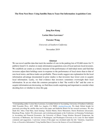
Satellite data sourcesNASA – Earthdata: https://earthdata.nasa.gov/ (requires free account)ESA Sentinel-5P – Copernicus Open Access Hub: https://s5phub.copernicus.eu/dhus/#/home(guest username/password for data access: s5pguest/s5pguest)NASA Global SO2 Monitoring: https://so2.gsfc.nasa.gov/ (daily SO2 maps of volcanic regionsfrom UV satellite instruments and a portal to various other sources of volcanic SO2 data)1. Web-based satellite data visualization with NASA WorldviewThis first exercise is a simple visualization of satellite data using NASA’s Worldview interface(https://worldview.earthdata.nasa.gov/). Worldview is an excellent tool for browsing andvisualizing available global satellite data for a given volcanic eruption (decades of satellite dataare available, updated within 3 hours of observation), though only minimal quantitative analysisis possible. Apart from visualization, its main utility is to identify available datasets which canthen be downloaded directly from Worldview or other source(s) for further analysis, if needed.a) Open NASA Worldview in a web-browser. This should open a global basemap for thecurrent day (change the date using the year/month/day counters in the lower left of thewindow, or the time slider along the bottom). The default base layers are ‘true-color’visible satellite images from the Moderate Resolution Imaging Spectroradiometer(MODIS) instruments aboard the NASA Terra ( 10:30 am and 10:30 pm local timeoverpass; available since 2000) and Aqua ( 1:30 pm and 1:30 am local time overpass;available since 2002) satellites, and the Visible Infrared Imaging Radiometer Suite(VIIRS) aboard the Suomi-NPP (or Joint Polar Satellite System, JPSS; 1:30 pm and 1:30 am local time overpass; available since late 2015) satellite. Coastlines and placelabels can be overlaid on these base images. Click and drag to move around and zoom in/out to focus on regions of interest.b) For this example, we will use the 13 February 2014 explosive eruption of Kelut (Java,Indonesia; lat: 7.93ºS, lon: 112.308ºE), although feel free to explore any other eruption ofinterest (e.g., from the Smithsonian Institution Global Volcanism Program database or thesupplied MSVOLSO2L4 database). The Smithsonian GVP report of the February 2014Kelut eruption, which started at 2300 local time ( 1600 UTC) on February 13, is here.You can also download a GRL paper describing some analysis of satellite data for theKelut eruption.The first step is to navigate to the relevant date in Worldview and find Java(Indonesia) on the map. Note that, since the eruption started late on February 13 (after theTerra/Aqua MODIS daytime overpasses), the eruption cloud does not appear on theFebruary 13 MODIS visible images. To visualize the eruption cloud in this case we can!2
use nighttime infrared (IR) Brightness Temperatures (also available from MODIS, VIIRSand many other satellite instruments).c) To add a new data layer in Worldview, click ‘ Add Layers’ and a menu will appearlisting available layers by ‘Hazards and Disasters’ or ‘Science Discipline’. The ‘AshPlumes’ collection provides access to several datasets useful for visualizing volcanicplumes, including sulfur dioxide (SO2) data, aerosol data (for volcanic ash) and thermalanomalies (sensitive to active lava).To add a Brightness Temperature layer, start typing ‘Brightness Temperature’ inthe search field and many options will appear. Check the ‘Brightness Temperature (Band31-Night)’ layer from Aqua/MODIS to add it to the display. This layer should now appearin the list of ‘Overlays’ in the top left of the window; these can be switched on or offusing the ‘eye’ icon, and the order of the layer ‘stack’ can also be changed by dragginglayers up or down (it is useful to have the coastlines and place labels at the top so they areoverlaid on all other layers). The thresholds and color palette for the layer can also bechanged.With the Brightness Temperatures displayed (which are from Aqua/MODIS at 1:30 am local time on February 14, 2.5 hrs after the Kelut eruption), the volcanicumbrella cloud should be visible as a large, dark (i.e., low temperature) feature over EastJava (other similar features in the region are probably thunderstorm clouds). The coldtemperatures are consistent with an opaque cloud at high altitudes. By moving the mouseover the cloud you can view the actual temperatures recorded on the scale bar. One wayof estimating volcanic cloud altitude is to compare the IR brightness temperatures withthe closest (in time and location) radiosonde atmospheric temperature sounding (e.g.,obtained from the University of Wyoming). Do you notice anything unusual about thetemperature distribution in the volcanic cloud (especially over the location of Kelut),relative to other cold clouds in the region?d) Other useful layers to add for this nighttime case are accessed under ‘Ash Plumes’ - ‘Sulfur Dioxide’:i. Aqua/AIRS Sulfur Dioxide (Night, Prata Algorithm)ii. Aura/MLS Sulfur Dioxide (147 hPa, Night)The IR Atmospheric Infrared Sounder (AIRS on NASA’s Aqua satellite) and MicrowaveLimb Sounder (MLS) instruments can detect volcanic SO2 at night (unlike the UVsensors, OMI and OMPS). Note the unusual ‘ring-like’ SO2 distribution in the AIRS SO2data which is due to high opacity (probably due to ice/ash) preventing SO2 retrieval in thecenter of the volcanic cloud (cloud transparency is required for SO2 retrieval). MLSprovides a coarse vertical profile of SO2 in the upper troposphere and stratosphere alongthe Aura satellite track – the MLS data in Worldview are for just one layer (147 hPapressure; 14 km altitude).!3
e) You can also add orbit tracks from various satellites to the data stack. The Cloud-AerosolLidar and Infrared Pathfinder Satellite Observation (CALIPSO) satellite (https://wwwcalipso.larc.nasa.gov/), which carries a space-borne Light Detection and Ranging(LiDAR) instrument, can measure the altitude of volcanic clouds directly if the satellitetrack intersects the plume. Although CALIPSO LiDAR data cannot be visualized inWorldview, the CALIPSO satellite tracks can be viewed to check for plume intersection,since the CALIPSO, Aqua, and Aura satellites orbit in NASA’s A-Train constellation andhave very similar overpass times (within 10 minutes).To add CALIPSO Orbital Tracks, click ‘ Add Layers’ and search for‘CALIPSO’, then check ‘CALIPSO Orbital Track & Overpass Time (Descending/Night)’to display the nighttime CALIPSO track (roughly coincident with the Aqua MODIS andAIRS data). Note that the CALIPSO track cuts directly through the young Kelut eruptioncloud, which is a rare occurrence!If you want to then go and find the corresponding CALIPSO browse imageshowing the LiDAR backscatter data, you need to note the CALIPSO overpass time fromWorldview ( 18:15 UTC on Feb 13 in this case), go to the CALIPSO website (https://www-calipso.larc.nasa.gov), and browse to Products - LIDAR Browse Images - Version 4 (Go) - Select date (Feb 13, 2014) - Search for the image panel correspondingto the 18:15 UTC overpass (orbital track maps are available to aid navigation). See ifyou can locate the Kelut volcanic cloud feature in the CALIPSO data and obtain anapproximate altitude.f) Note that all layers added to the stack are preserved as you navigate forward or backwardin time in Worldview. To visualize the dispersion of the Kelut eruption cloud insubsequent days, you need to add other data layers available in daytime under ‘AshPlumes’ including:i. Aura/OMI UV Aerosol Index (for volcanic ash)ii. Aqua/AIRS Sulfur Dioxide (Day, Prata Algorithm)iii. Aura/MLS Sulfur Dioxide (147 hPa, Day)iv. Aura/OMI Sulfur Dioxide (Upper Troposphere and Stratosphere)Note that Aura/OMI, Aura/MLS and Aqua/AIRS (daytime) measurements are roughlycoincident in time. Comparing these datasets provides some insight into the differentsensitivity to volcanic SO2 in the UV (OMI) and IR (AIRS).g) Finally, many of the visualized satellite datasets can be downloaded for further offlineanalysis using the ‘Data’ tab at the top left of the screen. Satellite datasets are typicallypackaged as entire satellite orbits ( 14-15 orbits per day for a typical polar-orbiting asset)or as ‘granules’ covering smaller geographic regions.2. Satellite data visualization/extraction with NASA Panoply!4
This exercise uses NASA’s free Panoply Data Viewer to visualize data. Panoply is less userfriendly than Worldview, but provides more control over plotting parameters and access to thefull range of variables provided in satellite data files (HDF or netCDF). As with Worldview,minimal quantitative analysis is possible with Panoply (its main function is to produce images)but data can be extracted for further analysis if needed.Panoply is a Java application that enables the user to plot raster images of geo-gridded (georeferenced) data from datasets in netCDF or HDF format. Depending on the type of dataavailable, Panoply can be used to create displays in a variety of ways: Plot longitude-latitude data as global maps or zonal averages, using any of over 40 global mapprojections Overlay continent outlines or masks on longitude-latitude plots, or just plot a particular region Display specific latitude-longitude or latitude-vertical arrays from larger multidimensionalvariables as slicesPanoply also functions as a tool for graphical data analysis and reporting of results by allowingthe user to: Combine two arrays in one plot by differencing, summing or averaging Use any of the 30 scale colorbars provided, or add a custom colorbar Save plots to disk as PNG or GIF imagesFor this example, we will use the 26-27 July 2018 eruption of Ambae (or Aoba, Vanuatu; lat:15.389ºS, lon: 167.835ºE), which produced significant SO2 emissions. This exercise uses twocurrent satellite SO2 datasets, from the ESA/Sentinel-5P TROPOMI instrument and the NASASuomi-NPP OMPS instrument. These are both UV instruments, but TROPOMI has higher spatialresolution and hence greater sensitivity to volcanic SO2. As before, feel free to explore any othereruption of interest (e.g., from the Smithsonian Institution Global Volcanism Program databaseor the supplied MSVOLSO2L4 database).To locate the relevant TROPOMI orbit covering the Ambae volcanic cloud and load it intoPanoply:a) Go to the Sentinel-5P Hub: https://s5phub.copernicus.eu/dhus/#/homeb) Drag the map to the area of interest (Vanuatu) and draw a box over and to the east ofVanuatu (to do this you need to activate ‘area mode’ using the box icon at top right of thewindow).c) Click the bars on the left of the Search window (top left) to bring up Advanced Searchoptions, and enter the following:a. Sensing period: start: 2018/07/27; stop: 2018/07/27b. Product Type: L2 SO2c. Timeliness: Reprocessing!5
Then click the magnifying glass icon to search. You will be prompted to login using theusername/password: s5pguest/s5pguest, then you may need to hit search again.d) The results should list 1or 2 TROPOMI orbits that intersect your search box. ‘Mousingover’ the results will illuminate the corresponding orbit on the map. The results also showa Download URL for each orbit – rather than downloading the files (which are quitelarge), you can copy this URL and paste it in the ‘Enter the URL of a remote dataset toopen:’ window in Panoply. You will be prompted to login to Sentinel Hub again(s5pguest/s5pguest) and then the remote dataset should load (may take some timedepending on connection speed).e) In case of problems, here’s the direct link to TROPOMI orbit for Ambae on July 27, 2018(Sentinel Hub): s('64ba1ebdcb68-416e-a45d-8ca7e4dd059a')/ valueOnce loaded into Panoply, the structure of the TROPOMI data files (HDF version 5) can beexplored in the ‘Datasets’ tab. There are many parameters stored in the files, but to plot a map ofSO2 select: value - PRODUCT - SUPPORT DATA - DETAILED RESULTS - sulfurdioxide total vertical column 15kmThen click ‘Create Plot’ or right-click on the variable to create a plot. Select the option ‘Create ageoreferenced Longitude-Latitude plot’, then ‘Create’. Plotting may take some time as the dataare being read remotely. A window should open with a plot of the TROPOMI orbit on a globalmap. To zoom in to the area of interest (Vanuatu) you need to hold ‘Command’ (on a Mac) anddraw a new box; zoom out using ‘Option-Command’ (or use the Plot menu).Tabs at the bottom of the plot window allow you to change various plotting parameters: Array(s) – checking the ‘Interpolate’ box produces a smoothed map; unchecking the boxdisplays the actual sensor ground-pixels.Scale – change the range of the plotted data (e.g., remove negative values by setting Minto zero); change the color table and caption. Note: the units of TROPOMI SO2 columnsare moles m-2; to convert these to the more commonly used Dobson Units (DU; 1 DU 2.69 1016 molecules cm-2 0.0285 g m-2 SO2) you would need to multiply by a scalingfactor of 2241.15, but unfortunately it is not easy to do this in Panoply.Map – change map projection; re-center the map (note that the July 27, 2018 eruptioncloud from Ambae straddles the International Date Line, so try centering on 180ºE); add agraticule and labels.Overlays – add coastlines and country borders (MWDB Coasts Countries 1.cnob ishigh-resolution data, useful for small regions).Contours – add contours to the data plot.Labels – Add/change plot title, footnotes etc.!6
When you are happy with the plot you can save it using File - Save Image As. (defaultformat is PNG). You can also export the maps as KMZ files (e.g., for display in Google Earthor GIS software). To export the actual data (e.g., for use in a spreadsheet or other dataanalysis tool), highlight the variable of choice in the ‘Datasets’ tab (Panoply – Sourceswindow) and use File - Export Data.You can now repeat this procedure to locate and load OMPS SO2 data for the same Ambaeeruption (hard copies of data files will also be provided):f) To search for the OMPS data yourself, you can use the NASA Earthdata portal (https://search.earthdata.nasa.gov/search?q OMPS NPP NMSO2 PCA L2), which requiresyou to register for a free account to download data. Then choose a region and date ofinterest, search for corresponding data granules (OMPS-NPP NMSO2*.h5 files) andeither download the data files or copy the access URLs from the ‘Information’ tab foreach granule for use in Panoply. Detailed instructions are not provided here but it is fairlyintuitive.g) Alternatively, here is the direct link to an OMPS SO2 data file for the Ambae eruptionthat you can use in Panoply (this also requires an Earthdata account for download,however: OMPS NPP NMSO2 PCA L2.1/2018/208/OMPS-NPP NMSO2-PCAL2 v1.1 2018m0727t013256 o34954 2018m0727t060604.h5h) Once you have the data file URL, you can paste it in the ‘Enter the URL of a remotedataset to open:’ window in Panoply as before. It will then appear in the ‘Datasets’window under the TROPOMI data file. Alternatively, you can load a local data file fromyour hard disk using File - Open i) To locate the SO2 variable, select OMPS-NPP NMSO2 - SCIENCE DATA - ColumnAmountSO2 STL (stratospheric SO2 column amount). Now you have twooptions: make a new plot window (- Create Plot) or combine the OMPS SO2 data withthe previously plotted TROPOMI data (- Combine Plot). In the latter case, you will beasked in which existing plot you should combine the variable. Then in the combined plotwindow, you can toggle between the TROPOMI and OMPS SO2 data using the Array(s)tab:a. Plot Map of Array 1 Only – TROPOMIb. Plot Map of Array 2 Only – OMPSAgain, unchecking ‘Interpolate’ shows the native satellite spatial resolution. This is usefulfor comparing the high resolution TROPOMI observations (3.5x7 km) with the lowerresolution OMPS (50x50 km). However, due to the different units used in the TROPOMI(mol m-2) and OMPS (DU) files, you need to change the scaling on the ‘Scale’ tab using‘Fit to Data’j) You may find it easier to open the OMPS SO2 data in a new plot window (- Create Plot)for a side-by-side comparison. Compare the sensitivity and extent of the Ambae SO2 cloud!7
as observed by TROPOMI and OMPS (which have similar overpass times at 1:30 pmlocal time).Additional activities: try searching for and loading adjacent TROPOMI and/or OMPS orbitsfrom the same day or subsequent days to increase spatial coverage (the Ambae SO2 cloud spreadover the southern Pacific Ocean in the 1-2 weeks after the eruption). You can also try visualizingthe OMPS UV Aerosol Index data (sensitive to volcanic ash) in Panoply, or visualizing theOMPS data (and other datasets) for the Ambae eruption in NASA Worldview as described in (1)above. TROPOMI data are not currently available in Worldview but can be visualized (alongwith many other ESA Sentinel datasets) in the similar Sentinel EO Browser (https://apps.sentinel-hub.com/eo-browser).More information on Panoply is available in these Documentation/Panoply ik/images/stories/pdf/visualizing netcdf howto?title Quick%20View%20Data%20with%20Panoply3. Online satellite data analysis using NASA GiovanniIn this final visualization exercise, we will explore the use of NASA’s Giovanni i) for online satellite data analysis. In contrast toWorldview and Panoply, which are primarily data visualization tools, Giovanni can be used toanalyze large amounts of satellite data online without downloading the files. Satellite dataanimations can also be generated. Here, we will use Giovanni to create a time-averaged map ofsatellite SO2 data to detect and visualize passive volcanic degassing. The only relevant satelliteSO2 dataset currently available in Giovanni is from the NASA Ozone Monitoring Instrument(OMI). Some generic instructions are provided below, but you are encouraged to exploredifferent volcanic regions and time periods to visualize the variability in volcanic degassing.Note: although limited functionality in Giovanni is available as a ‘guest user’, a free NASAEarthdata account provides full access.(a) From the Giovanni home page, various plot types are available under ‘Select Plot’ (e.g.,time-averages, cumulative plots, comparisons, vertical profiles, etc). Select the firstoption: ‘Maps: Time Averaged Map’.(b) Next, Select Date Range (UTC) for the time-averaging. This is your choice, but you maywant to experiment with annual, seasonal or monthly averages. Note that the OMI SO2dataset used for analysis is available from October 2004 to present. The stronger thevolcanic SO2 source, the less data averaging is required to ‘detect’ the source in satellitedata, and vice versa.!8
(c) Next, Select Region (Bounding Box or Shape) for analysis, using the ‘Draw boundingbox on map’ tool. Use the ‘hand’ to roam around the map, then zoom in to your region ofinterest and draw a box. The smaller the box, the faster the analysis will run. The choiceof region is up to you, but some global volcanic SO2 emission ‘hotspots’ include Vanuatu,Papua New Guinea, Hawaii (Kilauea), Mexico, Colombia/Ecuador, southern Peru, andSicily (Etna). More details on volcanic SO2 sources are here.(d) Now, Select Variables. Under ‘Measurements’, check the SO2 box. Four availabledatasets should appear in a Table. Select ‘SO2 Column Amount (Planetary BoundaryLayer) OMSO2e v003’, which is the OMI SO2 dataset. The other SO2 datasets listed aremodel output from the MERRA-2 Model (not actual observations), but you could also tryplotting these for comparison with the OMI SO2 data. In the model data, SO2 emissionsare simulated using emissions inventories.(e) Now hit ‘Plot Data’ in the bottom right of the window, and the data analysis will belaunched. This may take some time, depending on the selected time-period and size ofregion.(f) Once complete, a map of time-averaged OMI SO2 columns will appear. Various aspectsof the map can be changed using the ‘Options’ menu; e.g., change the scale, color palette,caption, title etc. Maps can also be downloaded as GeoTIFF, KMZ or PNG files.Unfortunately, volcano locations cannot be plotted – see which volcanoes you canidentify based on their SO2 emissions.(g) Further analysis using Giovanni could include comparison of annual or monthly meanSO2 maps for a particular volcano; e.g., Kilauea’s SO2 emissions increased significantlyafter the summit eruption in March 2008. You could also experiment with some othertools available in Giovanni (e.g., data animation).!9
Other exercisesCalculation of the sulfur budget for the 2011 Grimsvötn (Iceland) eruptionThis exercise is an example of a common problem in volcanic emission studies: inferring thetotal volcanic sulfur budget based on measured emissions of only 1 or 2 sulfur species.Goal: calculate the sulfur (S) budget of the May 2011 explosive eruption of Grimsvötn (Iceland)based on satellite remote sensing measurements of degassing and petrological data (Sconcentrations in the melt), and estimates of other sulfur sinks in the volcanic system.Satellite remote sensing data and derived estimate of other sulfur speciesThe following sulfur gas species were measured or estimated in the Grimsvötn eruption cloud[Sigmarsson et al., 2013]:0.3 Tg SO2 (OMI measurements)29 Gg H2S (IASI measurements)15 Gg S2 (estimated based on assumed gas ratios)1 Tg 1012 g1 Gg 109 gAsh leachate dataAn estimated 118 Gg S was sequestered on volcanic ash in the eruption column [Olsson et al.,2013]Petrological estimate of Grimsvötn SO2 emissionsDegassed SO2 mass 64ρV (S Sg)32 DRE iSi 0.1750 wt%Sg 0.0687 wt%VDRE 0.25 km3Where 64/32 ratio of molecular weights of SO2 and S; ρ 2750 kg m-3 (melt density); VDRE 0.25 km3 (eruption volume, Dense Rock Equivalent); Si initial S concentration (from meltinclusions); Sg residual S concentration after degassing (from groundmass).Other sulfur sinks!10
Other potential sinks for S in the Grimsvötn system are:S lost to hydrothermal system and caldera lake (Slake) 37 Gg SS conserved in the magma as sulfide globules (Ssulfide globules). Sulfide globules were observed inthe erupted products.Total S mass balance for 2011 Grimsvötn eruptionSi – (Sg Ssatellite Sleachate Slake Ssulfide globules) 0Step 1: calculate the total eruptive S emission (as SO2, H2S and S2) based on satellitemeasurements.Step 2: estimate the total S emission, accounting for the S scavenged in the eruption column.What proportion of the emitted S was scavenged and returned to the ground in ashfall?Step 3: calculate the petrological estimate of SO2 emissions, and compare this with the satelliteobservations.Step 4: estimate the amount and proportion of the total S budget conserved in the magma assulfide globules, according to the mass balance equation provided.ReferencesOlsson, J., S. L. S. Stipp, K. N. Dalby, and S. R. Gislason (2013), Rapid release of metal salts andnutrients from the 2011 Grímsvötn, Iceland volcanic ash, Geochim. Cosmochim. Acta, 123, 134–149, doi:10.1016/j. gca.2013.09.009.Sigmarsson, O., B. Haddadi, S. Carn, S. Moune, J. Gudnason, K. Yang, and L. Clarisse (2013), The sulfurbudget of the 2011 Grímsvötn eruption, Iceland, Geophys. Res. Lett., 40, doi:10.1002/2013GL057760.!11
Hence, most users of satellite data write their own codes for analysis (e.g., in IDL, Matlab, Python etc.). The most common satellite data formats are Hierarchichal Data Format (HDF, HDF4, HDF5, etc.) and the related Network Common Data Form (NetCDF) and most programming langua