Transcription
KMV Model
Expected default frequency Expected default frequency (EDF) is a forward-looking measureof actual probability of default. EDF is firm specific. KMV model is based on the structural approach to calculate EDF(credit risk is driven by the firm value process).–It is best when applied to publicly traded companies, where thevalue of equity is determined by the stock market.–The market information contained in the firm’s stock priceand balance sheet are translated into an implied risk of default.
Distribution of terminal firm valueat maturity of debt σ V2 VT V0 exp µ 2 firm value T σ V T Z T V0par valuedefault regiontimeT According to KMV’s empirical studies, log-asset returns confirmquite well to a normal distribution, and σV stays relatively constant.
Three steps to derive the actual probabilities of default:1. Estimation of the market value and volatility of the firm’s asset.2. Calculation of the distance to default, an index measure of defaultrisk.3. Scaling of the distance to default to actual probabilities of defaultusing a default database.
Estimation of firm value V andvolatility of firm value σV Usually, only the price of equity for most public firms is directlyobservable, and in some cases, part of the debt is directly traded. Using option pricing approach:equity value, E f(V, σV, K, c, r)andvolatility of equity, σE g(V, σV, K, c, r)where K denotes the leverage ratio in the capital structure, c is theaverage coupon paid on the long-term debt, r is the riskfree rate. Solve for V and σE from the above 2 equations.
Distance to defaultdefault point,d*1 short-term debt long-term debt2distance to default,E (VT ) d *df σV (ln d * µ V0σˆ V Tσˆ V22)T ,where V0 is the current market value of firm, µ is the expected netreturn on firm value and σ̂ V is the annualized firm value volatility.
Probabilities of default fromthe default distanceEDF40 bpdefault distance123456Based on historical information on a large sample of firms, for eachtime horizon, one can estimate the proportion of firms of a givendefault distance (say, df 4.0) which actually defaulted after oneyear.
ExampleCurrent market value of assetsNet expected growth of assets per annum*Expected asset value in one yearAnnualized asset volatilityDefault pointdefault distance, d f V0 1,000µ 20%VT 1,200σV 100d* 8001,200 800 4.100Among the population of all the firms with df 4 at one point in time,say 5,000 firms, 20 defaulted in one year. Then20EDF1- yr 0.004 40bp.5,000*KMV Credit Monitor uses a constant asset growth assumption for all firms in thesame market.
Example Federal Express(dollars in billions of US )Market capitalization(price shares outstanding)Book liabilitiesMarket value of assetsAsset volatilityDefault pointDefault distanceEDFNovember 1997 7.9February 1998 7.3 4.7 12.615% 3.412 .6 3 .4 4 .90 .15 12 .60 .06 %( 6 bp ) AA 4.9 12.217% 3.512 .2 3 .5 4 .20 .17 12 .20 .11 %(11 bp ) A The causes of changes for an EDF are due to variations in the stockprice, debt level (leverage ratio), and asset volatility.
Key features in KMV model1. Dynamics of EDF comes mostly from the dynamics of the equityvalues.2. Distance to default ratio determines the level of default risk. This key ratio compares the firm’s net worth to its volatility. The net worth is based on values from the equity market, so itis both timely and superior estimate of the firm value.3. Ability to adjust to the credit cycle and ability to quickly reflect anydeterioration in credit quality.4. Work best in highly efficient liquid market conditions.
Strength of KMV approach Changes in EDF tend to anticipate at least one year earlier than thedowngrading of the issuer by rating agencies like Moody’s andS & P’s. EDF provides a cardinal rather than ordinal ranking of credit quality.
Accurate and timely information from the equity market providesa continuous credit monitoring process that is difficult andexpensive to duplicate using traditional credit analysis. Annual reviews and other traditional credit processes cannotmaintain the same degree of vigilance that EDFs calculated ona monthly or a daily basis can provide.
Weaknesses of KMV approach It requires some subjective estimation of the input parameters. It is difficult to construct theoretical EDF’s without the assumptionof normality of asset returns. Private firms’ EDFs can be calculated only by using somecomparability analysis based on accounting data. It does not distinguish among different types of long-term bondsaccording to their seniority, collateral, covenants, or convertibility.
ExampleValuation of a zero coupon bond with a promised payment in a year of 100, with a recovery of (1 LGD) upon issuer’s default.*LGD loss given default (assumed to be 40% here)Q risk neutral probability that the issuer defaults in one year fromnow (assumed to be 20% here)The expectation is calculated using the risk neutral probabilities butnot the actual probabilities as they can be observed in the market fromhistorical data or EDFs.
100(1 LGD) 100Q 1Qrisky bond1 Q 1no defaultdefault 100(1 LGD) 100 LGDQ Q 100(1 LGD)default free componentQ0risky component
PV1 PV(risk-free cash flow) 100 (1 LGD)/(1 r) 54.5r risk free rate (assumed to be 10% here)PV2 PV (risky cash flow) EQ (discounted risky cash flow)100LGD(1 Q ) 0 Q 29.1.1 rLet s denote the credit spread100(1 LGD ) 100 LGD (1 Q )100 1 r1 r1 r sso thatLGD Qs (1 r ) 9.6%.1 LGD Q
Derivation ofthe risk neutral EDFsLet VT* be the firm value process at T under the modified riskneutral process.dVt* rdt σdZ t*VtQ Pr [VT* DPTT ] σ2 T σ T Z T ln DPTT Pr ln V0 r 2 2V0σ ln DPTT r 2 T * Pr ZT N ( d 2 )σ T [whered *2ln)](V0DPTT( r σ Tσ22)T .
On the other hand, the expected default frequency under the actualprocess is given byEDFT N ( d 2 )whereV0σ2ln DPTT µ 2 Td2 .σ T()Hence, the risk neutral EDFµ r 1 Q N N ( EDFT ) T .σ From CAPM, we haveµ r β (µ M r ) ρ FM σ(µ M r )σMwhere β beta of the asset with the market portfolioµM r market risk premium for one unit of beta risk(to be estimated by a separate statistical process).
* KMV Credit Monitor uses a constant asset growth assumption for all firms in the same market.