Transcription
TM1TM2337TM3TM4TM5TM6Dr. Robert A. SchowengerdtTM7Landsat Thematic Mapper (TM) multispectralimages of desert and agriculture near Yuma,ArizonaMULTISPECTRAL IMAGE PROCESSING ISENSORSMultispectralrelatively low spectral resolution(typically 50–100nm) and smallnumber (typically 5-10) ofdiscrete spectral bandstypically acquired with multipath or multiple, filtered opticalsystemsfirst satellite multispectralsensor was Landsat in 1972Landsat image size 250MBCommon “color” images, e.g.video or camera photos, are 3band examples of multispectralimagesECE/OPTI533 Digital Image Processing class notes2003
338vegetation appears red ,soil appears yellow - grey,water appears blue - blackDr. Robert A. Schowengerdt2003red color assigned to near IR sensor bandgreen color assigned to red sensor bandblue color assigned to green sensor bandFor example, Color InfraRed (CIR)composite uses:MULTISPECTRAL IMAGE PROCESSING ICombine band images in color composite forinterpretationECE/OPTI533 Digital Image Processing class notes
Dr. Robert A. Schowengerdt2003AvIRIS hyperspectral image cube ofLos Alamos, NM (courtesy ChrisBorel, LANL)MULTISPECTRAL IMAGE PROCESSING IHyperspectralrelatively high spectral resolution (typically5–10nm) and large number (typically 200) ofnearly-contiguous bandstypically acquired with an imagingspectrometer over the wavelength range 400to 2400nmhigh spectral resolution potentially allowshigh discrimination of surface featuresprimarily airborne - e.g. Airborne VisibleInfraRed Imaging Spectrometer (AVIRIS)operated by NASA/JPL, 1989 - date339first satellite hyperspectral sensor is Hyperionon NASA EO-1, 2000 - dateHyperion image size 1.1GBECE/OPTI533 Digital Image Processing class notes
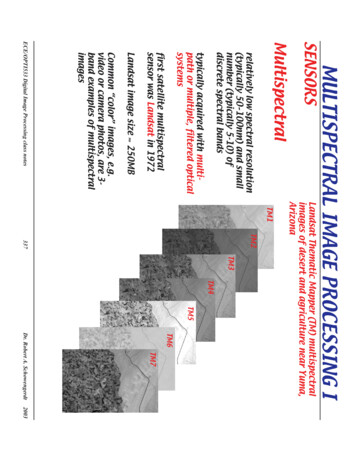
2400grasssoilwaterDr. Robert A. SchowengerdtbuildingMULTISPECTRAL IMAGE PROCESSING Isoilgrassbuildingwater2000340Feature discrimination using hyperspectral imagery800Airborne Visible-InfraRed Imaging Spectrometer (AVIRIS) ofPalo Alto, CA2500200015001000500040012001600wavelength (nm)ECE/OPTI533 Digital Image Processing class notesDN2003
2CO2H O0.8H O22CO ,2H O1.21.6wavelength (µ m)2CO ,2H O2COCO222H O2.4341Dr. Robert A. SchowengerdtMULTISPECTRAL IMAGE PROCESSING I0.4Spectral movie of AVIRIS image, Palo Alto, CA10.80.60.40.20ECE/OPTI533 Digital Image Processing class notestransmittance2003
MULTISPECTRAL IMAGE PROCESSING IDATA REPRESENTATION[K] DN ij1 DN ij2 DN ijKDN ij1DN ij2T342Dr. Robert A. Schowengerdt K-dimensional space formed by DNs in K spectral bands of amulti- or hyperspectral imageDN ij K-dimensional column vectorpixel at (i,j): DN ijKECE/OPTI533 Digital Image Processing class notes2003
DNp3DN3DN pDN p1 DN p2DN p3DNp2Dr. Robert A. Schowengerdt2003With 200 bands and 11 bits/pixel,number of possible data vectors 2048200With 3 bands and 8 bits/pixel,number of possible data vectors2563 16,777,216 Data space is quantizedinto (2Q)K volumeelements, or “bins” In three dimensions, eachpixel plots as a vectorMULTISPECTRAL IMAGE PROCESSING IDNp1DN2343Example multsipectral data vector at pixel p for3-bandsDN1ECE/OPTI533 Digital Image Processing class notes
Dr. Robert A. SchowengerdtMULTISPECTRAL IMAGE PROCESSING IK-dimensional histogramhist DN count ( DN ) N PDF ( DN )344 the value of histDN at a particularDN vector is the number of pixelsthat have that vector scalar function of a vectorECE/OPTI533 Digital Image Processing class notes2003
MULTISPECTRAL IMAGE PROCESSING 35040005031000DN50DN4pixelsScattergrams and N3 Scattergram is greylevel visualization of K-D histogram16001400600DN4pixelsscattergram in 2-D140012006004008004002000pixelsECE/OPTI533 Digital Image Processing class notes345Dr. Robert A. SchowengerdtNote, the “features” in scatter-space, corresponding to objects in image 1200pixelsDN32003
3461801601401201000001010203040DN3 502060 0 6 DN4 50 6 0 50 60 7007 7700 3040DN32050503050202030402DN30402DN60DN24060 040DN3DN4DN4Dr. Robert A. Schowengerdt2003Example for K 3 viewed from different directionsMULTISPECTRAL IMAGE PROCESSING I Scatterplot is a binaryplot of the K-DhistogramECE/OPTI533 Digital Image Processing class notesDN4DN4
201001401601801201401601802040608010 01201008060402000010180160140120100203040DN310 707 60 50 6040DN230505030402DN60 2020 040200DN40101801601401208010060402002003040DN3 707 60 50 2040DN330505060 30402DN 102070100160140120100806040200Dr. Robert A. Schowengerdtband 4 vs band 3180MULTISPECTRAL IMAGE PROCESSING I30402DNDN4806040200060 2-D scatterplot obtained by projecting 3-D scatterplot5070 can also be obtained by thresholding the 2-D scattergram6060DN4 707 60 nd 4 vs band 2347DN412010 0806040200DN3302010010 band 3 vs band 20 ECE/OPTI533 Digital Image Processing class notesDN42003
34563487654321Dr. Robert A. Schowengerdt2003All possible 2-Dscatterplots for a 7band Landsat TM imageMULTISPECTRAL IMAGE PROCESSING I2ECE/OPTI533 Digital Image Processing class notes
N DN p NT 〈 DN 〉Dr. Robert A. SchowengerdtMULTISPECTRAL IMAGE PROCESSING ISpectral Covariance and Correlation Multivariate DN mean vectorµp 1 Multivariate DN covariance matrixCc 11 c 1KT 〈 ( DN – µ ) ( DN – µ ) 〉c K1 c KKN ( DNpm – µm ) ( DNpn – µn )349c kk (N – 1)Elements are covariance between bands m and n:c mn p 1Diagonal elements are variance of band kECE/OPTI533 Digital Image Processing class notes2003
DNhigh correlationmmoderate correlationno correlationρmnρmn 1mmnnnDN c0 ρ mn 1 0, cρmn –1 0, cmm c0 ρ mn – 1mnDr. Robert A. Schowengerdtρscatterplot shape and correlationMULTISPECTRAL IMAGE PROCESSING I Multivariate DN correlation matrixRρ mn ρ nm3501 ρ 1K , – 1 ρ mn 1 or ρ mn 1ρ K1 11 2Correlation between bands m and n:ρ mn c mn ( c mm c nn )Normalized by variance in each band Special properties of covarianceand correlation matricesandC and R are symmetric, i.e.,c mn c nmIf C and R are diagonal, the pixel values inbands m and n are uncorrelatedECE/OPTI533 Digital Image Processing class notesnn2003
MULTISPECTRAL IMAGE PROCESSING IPrincipal Component Transform AKA Karhunen-Loeve or Hotelling transform linear matrix transform PC W PC DNwhere:PC is the K–dimensional principal component vectorWPC is a K x K transformation matrixDN is the original multi- or hyperspectral pixel vector351Dr. Robert A. Schowengerdt each principal component is a weighted average of all spectralbandsECE/OPTI533 Digital Image Processing class notes2003
MULTISPECTRAL IMAGE PROCESSING ITdiagonalizes the covariance matrix, C, of the original image, Properties of the PCTW PCC PCC PCare the eigenvalues of the datais diagonal, the PC components are uncorrelatedC PC W PC CW PCsinceThe diagonal elements ofC PCC – λk I 0λ k , is equal to the variance of the kth PC and is found byλ1 0eigenvalue 1 0 0 eigenvalue K0 λKeach eigenvalue,solving the characteristic equation,352Dr. Robert A. SchowengerdtNote, trace of Cpc equals trace of C, i.e. the sum of the eigenvalues equals thesum of the original image band variancesECE/OPTI533 Digital Image Processing class notes2003
MULTISPECTRAL IMAGE PROCESSING Iteigenvector 1: te1:teKe 11 e 1K ::e K1 e KKW PC consists of the eigenvectors of the data along its rows,W PC tDr. Robert A. Schowengerdt2003e k , consists of the weights applied to the original bands to obtaineigenvector Keach eigenvector,353the kth PC and is found by solving the equation,( C – λ k I )e k 0ECE/OPTI533 Digital Image Processing class notes
45C – λk I 0Characteristic Equation1 0.761R 0.761 1C 1.9 1.11.1 1.1µ 3.503.50MULTISPECTRAL IMAGE PROCESSING I3DN2DN1DN12which has solutions2pixel23λ 2.671124Example Data5432100233 03441.9 – λ 1.11.1 1.1 – λ455andDr. Robert A. Schowengerdtλ 0.33λ – 3λ 0.88 02553546ECE/OPTI533 Digital Image Processing class notesDN22003
2.67 00 0.33MULTISPECTRAL IMAGE PROCESSING I ThereforeC PC2Dr. Robert A. Schowengerdt2003, which are not independent.Note that PC1 accounts for 2.67/3 0.89 of total variance in data Find eigenvectors using ( C – λ k I )e k 0– 0.77e 11 1.10e 12 01.10e 11 – 1.57e 12 0e 11 1.43e 12For example, for eigenvector e1From either equation2 Eigenvectors are orthogonal unit vectors implies e 11 e 12 1 . Solving simultaneously with above equation gives eigenvector355e 1 0.82 and, with a similar analysis, eigenvector e 2 – 0.570.570.82ECE/OPTI533 Digital Image Processing class notes
0.82 0.57– 0.57 0.82Dr. Robert A. SchowengerdtMULTISPECTRAL IMAGE PROCESSING I Final transformation matrixW PC356Find and plot newcoordinates of data pointsin PC spaceECE/OPTI533 Digital Image Processing class notes2003
PC1DN1TM bandsPC bands56Dr. Robert A. SchowengerdtMULTISPECTRAL IMAGE PROCESSING I Why use the PCT?235734band or PC indexλ1 λ2 λKDecorrelates the spectral data optimallyDN2PC21Compresses the variance8006004002000ECE/OPTI533 Digital Image Processing class notesDN variance2003
Dr. Robert A. SchowengerdtMULTISPECTRAL IMAGE PROCESSING I Why not use the PCT?data-dependent W coefficients change from scene-to-scene Makes consistent interpretation of PC imagesdifficultspectral details, particularly in small areas,may be lost if higher-order PCs are ignored358computationally expensive for large imagesor for many spectral bandsECE/OPTI533 Digital Image Processing class notes2003
TM1 TM2 TM3 TM4 TM6 TM7 SENSORS Multispectral relatively low spectral resolution . Hyperion on NASA EO-1, 2000 - date Hyperion image size 1.1GB AvIRIS hyperspectral image cube of Los Alamos, N